*** QuickLaTeX cannot compile formula:
"><code>colStats()</code></a> 方法返回一个 <a href="http://spark.apache.org/docs/1.6.2/api/scala/index.html#org.apache.spark.mllib.stat.MultivariateStatisticalSummary"><code>MultivariateStatisticalSummary</code></a>的实例,其中包含每列的最大值、最小值、均值等等。这里简单的列出了一些基本的统计结果。
<pre><code class="scala">scala> val summary: MultivariateStatisticalSummary = Statistics.colStats(observations)
summary: org.apache.spark.mllib.stat.MultivariateStatisticalSummary = org.apache.spark.mllib.stat.MultivariateOnlineSummarizer@1a5462ad
scala> println(summary.mean)
[3.7586666666666666,1.1986666666666668]
scala> println(summary.variance)
[3.113179418344516,0.5824143176733783]
scala> println(summary.numNonzeros)
[150.0,150.0]
</code></pre>
用case class定义一个schema:Iris,Iris就是需要的数据的结构;然后读取数据,创建一个Iris模式的RDD,然后转化成dataframe;最后调用show()方法来查看一下部分数据。
<pre><code class="scala">scala> case class Iris(features: Vector, label: String)
defined class Iris
scala> val data = sc.textFile("G:/spark/iris.data")
| .map(_.split(","))
| .map(p => Iris(Vectors.dense(p(2).toDouble, p(3).toDouble), p(4).toString()))
| .toDF()
data: org.apache.spark.sql.DataFrame = [features: vector, label: string]
scala> data.show()
+---------+-----------+
| features| label|
+---------+-----------+
|[1.4,0.2]|Iris-setosa|
|[1.4,0.2]|Iris-setosa|
|[1.3,0.2]|Iris-setosa|
|[1.5,0.2]|Iris-setosa|
|[1.4,0.2]|Iris-setosa|
|[1.7,0.4]|Iris-setosa|
|[1.4,0.3]|Iris-setosa|
|[1.5,0.2]|Iris-setosa|
|[1.4,0.2]|Iris-setosa|
|[1.5,0.1]|Iris-setosa|
|[1.5,0.2]|Iris-setosa|
|[1.6,0.2]|Iris-setosa|
|[1.4,0.1]|Iris-setosa|
|[1.1,0.1]|Iris-setosa|
|[1.2,0.2]|Iris-setosa|
|[1.5,0.4]|Iris-setosa|
|[1.3,0.4]|Iris-setosa|
|[1.4,0.3]|Iris-setosa|
|[1.7,0.3]|Iris-setosa|
|[1.5,0.3]|Iris-setosa|
+---------+-----------+
only showing top 20 rows
</code></pre>
有的时候不需要全部的数据,比如ml库中的logistic回归目前只支持2分类,所以要从中选出两类的数据。这里首先把刚刚得到的数据注册成一个表iris,注册成这个表之后,就可以通过sql语句进行数据查询,比如这里选出了所有不属于``Iris-setosa''类别的数据。选出需要的数据后,把结果打印出来看一下,这时就已经没有``Iris-setosa''类别的数据。
<pre><code class="scala">scala> data.registerTempTable("iris")
scala> val df = sqlContext.sql("select * from iris where label != 'Iris-setosa'")
df: org.apache.spark.sql.DataFrame = [features: vector, label: string]
scala> df.map(t => t(1)+":"+t(0)).collect().foreach(println)
Iris-versicolor:[4.7,1.4]
Iris-versicolor:[4.5,1.5]
Iris-versicolor:[4.9,1.5]
Iris-versicolor:[4.0,1.3]
Iris-versicolor:[4.6,1.5]
Iris-versicolor:[4.5,1.3]
... ...
</code></pre>
<h5>3. 构建ML的pipeline</h5>
分别获取标签列和特征列,进行索引,并进行了重命名。
<pre><code class="scala">scala> val labelIndexer = new StringIndexer().setInputCol("label").setOutputCol("indexedLabel").fit(df)
labelIndexer: org.apache.spark.ml.feature.StringIndexerModel = strIdx_a14ddbf05040
scala> val featureIndexer = new VectorIndexer().setInputCol("features").setOutputCol("indexedFeatures").fit(df)
featureIndexer: org.apache.spark.ml.feature.VectorIndexerModel = vecIdx_755d3f41691a
</code></pre>
接下来,把数据集随机分成训练集和测试集,其中训练集占70%。
<pre><code class="scala">scala> val Array(trainingData, testData) = df.randomSplit(Array(0.7, 0.3))
trainingData: org.apache.spark.sql.DataFrame = [features: vector, label: string]
testData: org.apache.spark.sql.DataFrame = [features: vector, label: string]
</code></pre>
然后,设置logistic的参数,这里我们统一用setter的方法来设置,也可以用ParamMap来设置(具体的可以查看spark mllib的官网)。这里设置了循环次数为10次,正则化项为0.3等,具体的可以设置的参数可以通过explainParams()来获取,还能看到程序已经设置的参数的结果。
<pre><code class="scala">scala> val lr = new LogisticRegression().
| setLabelCol("indexedLabel").
| setFeaturesCol("indexedFeatures").
| setMaxIter(10).
| setRegParam(0.3).
| setElasticNetParam(0.8)
lr: org.apache.spark.ml.classification.LogisticRegression = logreg_a58ee56c357f
scala> println("LogisticRegression parameters:\n" + lr.explainParams() + "\n")
LogisticRegression parameters:
elasticNetParam: the ElasticNet mixing parameter, in range [0, 1]. For alpha = 0, the penalty is an L2 penalty. For alpha = 1, it is an L1 penalty (default: 0.0, current: 0.8)
featuresCol: features column name (default: features, current: indexedFeatures)
fitIntercept: whether to fit an intercept term (default: true)
labelCol: label column name (default: label, current: indexedLabel)
maxIter: maximum number of iterations (>= 0) (default: 100, current: 10)
predictionCol: prediction column name (default: prediction)
probabilityCol: Column name for predicted class conditional probabilities. Note: Not all models output well-calibrated probability estimates! These probabilities should be treated as confidences, not precise probabilities (default: probability)
rawPredictionCol: raw prediction (a.k.a. confidence) column name (default: rawPrediction)
regParam: regularization parameter (>= 0) (default: 0.0, current: 0.3)
standardization: whether to standardize the training features before fitting the model (default: true)
threshold: threshold in binary classification prediction, in range [0, 1] (default: 0.5)
thresholds: Thresholds in multi-class classification to adjust the probability of predicting each class. Array must have length equal to the number of classes, with values >= 0. The class with largest value p/t is predicted, where p is the original probability of that class and t is the class' threshold. (undefined)
tol: the convergence tolerance for iterative algorithms (default: 1.0E-6)
weightCol: weight column name. If this is not set or empty, we treat all instance weights as 1.0. (default: )
</code></pre>
这里设置一个labelConverter,目的是把预测的类别重新转化成字符型的。
<pre><code class="scala">scala> val labelConverter = new IndexToString().
| setInputCol("prediction").
| setOutputCol("predictedLabel").
| setLabels(labelIndexer.labels)
labelConverter: org.apache.spark.ml.feature.IndexToString = idxToStr_89b2b1508b35
</code></pre>
构建pipeline,设置stage,然后调用fit()来训练模型。
<pre><code class="scala">scala> val pipeline = new Pipeline().
| setStages(Array(labelIndexer, featureIndexer, lr, labelConverter))
pipeline: org.apache.spark.ml.Pipeline = pipeline_33fa7f88685a
scala> val model = pipeline.fit(trainingData)
model: org.apache.spark.ml.PipelineModel = pipeline_33fa7f88685a
</code></pre>
pipeline本质上是一个评估器(Estimator),当pipeline调用fit()的时候就产生了一个PipelineModel,本质上是一个转换器(Transformer)。然后这个PipelineModel就可以调用transform()来进行预测,生成一个新的DataFrame,即利用训练得到的模型对测试集进行验证。
<pre><code class="scala">scala> val predictions = model.transform(testData)
predictions: org.apache.spark.sql.DataFrame = [features: vector, label: string,
indexedLabel: double, indexedFeatures: vector, rawPrediction: vector, probabilit
y: vector, prediction: double, predictedLabel: string]
</code></pre>
最后输出预测的结果,其中select选择要输出的列,collect获取所有行的数据,用foreach把每行打印出来。
<pre><code class="scala">scala> predictions.
| select("predictedLabel", "label", "features", "probability").
| collect().
| foreach { case Row(predictedLabel: String, label: String, features: Vector, prob: Vector) =>
| println(s"(
*** Error message:
Unicode character 方 (U+65B9)
leading text: $"><code>colStats()</code></a> 方
Unicode character 法 (U+6CD5)
leading text: $"><code>colStats()</code></a> 方法
Unicode character 返 (U+8FD4)
leading text: $"><code>colStats()</code></a> 方法返
Unicode character 回 (U+56DE)
leading text: $"><code>colStats()</code></a> 方法返回
Unicode character 一 (U+4E00)
leading text: $"><code>colStats()</code></a> 方法返回一
Unicode character 个 (U+4E2A)
leading text: ...de>colStats()</code></a> 方法返回一个
You can't use `macro parameter character #' in math mode.
leading text: ...apache.org/docs/1.6.2/api/scala/index.html#
Unicode character 的 (U+7684)
leading text: ...ultivariateStatisticalSummary</code></a>的
Unicode character 实 (U+5B9E)
label,  prob, predictedLabel=$predictedLabel")
| }
(Iris-versicolor, [3.5,1.0]) --> prob=[0.6949117083297265,0.30508829167027346], predictedLabel=Iris-versicolor
(Iris-versicolor, [4.1,1.0]) --> prob=[0.694606868968713,0.30539313103128685], predictedLabel=Iris-versicolor
(Iris-versicolor, [4.3,1.3]) --> prob=[0.6060637422536634,0.3939362577463365], predictedLabel=Iris-versicolor
(Iris-versicolor, [4.4,1.4]) --> prob=[0.5745401752760255,0.4254598247239745], predictedLabel=Iris-versicolor
(Iris-versicolor, [4.5,1.3]) --> prob=[0.6059493387519529,0.39405066124804705],
predictedLabel=Iris-versicolor
(Iris-versicolor, [4.5,1.5]) --> prob=[0.5423986730485701,0.45760132695142974],
... ...
4. 模型评估
创建一个MulticlassClassificationEvaluator实例,用setter方法把预测分类的列名和真实分类的列名进行设置;然后计算预测准确率和错误率。
scala> val evaluator = new MulticlassClassificationEvaluator().
     |       setLabelCol("indexedLabel").
     |       setPredictionCol("prediction")
evaluator: org.apache.spark.ml.evaluation.MulticlassClassificationEvaluator = mc
Eval_198b7e595a62
scala> val accuracy = evaluator.evaluate(predictions)
accuracy: Double = 0.9411764705882353
scala> println("Test Error = " + (1.0 - accuracy))
Test Error = 0.05882352941176472
从上面可以看到预测的准确性达到94.1%,接下来可以通过model来获取训练得到的逻辑斯蒂模型。前面已经说过model是一个PipelineModel,因此可以通过调用它的stages来获取模型,具体如下:
scala> val lrModel = model.stages(2).asInstanceOf[LogisticRegressionModel]
lrModel: org.apache.spark.ml.classification.LogisticRegressionModel = logreg_a58ee56c357f
scala> println("Coefficients: " + lrModel.coefficients+"Intercept: "+lrModel.intercept+
     |         "numClasses: "+lrModel.numClasses+"numFeatures: "+lrModel.numFeatures)
Coefficients: [0.0023957582955816056,0.13015697498232498]Intercept: -0.8315687375527291numClasses: 2numFeatures: 2


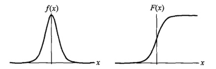
![\[F(x)=P(x \le x)=\frac 1 {1+e^{-(x-\mu)/\gamma}}\]](https://dblab.xmu.edu.cn/blog/wp-content/ql-cache/quicklatex.com-9f354d64015b505f718cd9ec4f98890e_l3.png "Rendered by QuickLaTeX.com")
![\[f(x)=F^{'}(x)=\frac {e^{-(x-\mu)/\gamma}} {\gamma(1+e^{-(x-\mu)/\gamma})^2}\]](https://dblab.xmu.edu.cn/blog/wp-content/ql-cache/quicklatex.com-5e9ba7a182194723ea58568d27bb2301_l3.png "Rendered by QuickLaTeX.com")
![\[\mu\]](https://dblab.xmu.edu.cn/blog/wp-content/ql-cache/quicklatex.com-75c83eedd5141ba143a525ba7949c2ae_l3.png "Rendered by QuickLaTeX.com")
![\[\gamma\]](https://dblab.xmu.edu.cn/blog/wp-content/ql-cache/quicklatex.com-9df94356151401c13b3565eab38aa533_l3.png "Rendered by QuickLaTeX.com")
![\[f(x)\]](https://dblab.xmu.edu.cn/blog/wp-content/ql-cache/quicklatex.com-f711bdb612e16efa1e06ed33178a159d_l3.png "Rendered by QuickLaTeX.com")
![\[F(x)\]](https://dblab.xmu.edu.cn/blog/wp-content/ql-cache/quicklatex.com-52866ddba463128c071bba7cfdc18c46_l3.png "Rendered by QuickLaTeX.com")
![\[(\mu, \frac 1 2)\]](https://dblab.xmu.edu.cn/blog/wp-content/ql-cache/quicklatex.com-4a760e6ab4e5a799ec3cb12f96c044b3_l3.png "Rendered by QuickLaTeX.com")
![\[P(Y=1|x)=\frac {exp(w \cdot x + b)} {1 + exp(w \cdot x + b)}\]](https://dblab.xmu.edu.cn/blog/wp-content/ql-cache/quicklatex.com-0fbac46d9cb25d3da0c5e0ce2491aa6e_l3.png "Rendered by QuickLaTeX.com")
![\[P(Y=0|x)=\frac {1} {1 + exp(w \cdot x + b)}\]](https://dblab.xmu.edu.cn/blog/wp-content/ql-cache/quicklatex.com-44fa7f0601e3607fabfda93ae964be51_l3.png "Rendered by QuickLaTeX.com")
![\[x \in R^n\]](https://dblab.xmu.edu.cn/blog/wp-content/ql-cache/quicklatex.com-477e1cd490f7330c49621f5e744e5038_l3.png "Rendered by QuickLaTeX.com")
![\[Y \in {0,1}\]](https://dblab.xmu.edu.cn/blog/wp-content/ql-cache/quicklatex.com-fcb9be84a0978a9b5f986ea8e23c1de4_l3.png "Rendered by QuickLaTeX.com")
![\[w \cdot x\]](https://dblab.xmu.edu.cn/blog/wp-content/ql-cache/quicklatex.com-f645be27f6922dcf5e963e9d3d41d4fb_l3.png "Rendered by QuickLaTeX.com")
![\[P(Y=1|x)=\pi (x), \quad P(Y=0|x)=1-\pi (x)\]](https://dblab.xmu.edu.cn/blog/wp-content/ql-cache/quicklatex.com-a8f70fd9541936adb9a5dbefb48231e4_l3.png "Rendered by QuickLaTeX.com")
![\[\prod_{i=1}^N [\pi (x_i)]^{y_i} [1 - \pi(x_i)]^{1-y_i}\]](https://dblab.xmu.edu.cn/blog/wp-content/ql-cache/quicklatex.com-f5d63ea80a9fd78a9f6a3841b41b955c_l3.png "Rendered by QuickLaTeX.com")
![\[L(w) = \sum_{i=1}^N [y_i \log{\pi(x_i)} + (1-y_i) \log{(1 - \pi(x_i)})]\]](https://dblab.xmu.edu.cn/blog/wp-content/ql-cache/quicklatex.com-7b5b46100544dfadefe100d2f5ce9736_l3.png "Rendered by QuickLaTeX.com")
![\[L(w)\]](https://dblab.xmu.edu.cn/blog/wp-content/ql-cache/quicklatex.com-71661cb137bd34c6ab95ab635582a958_l3.png "Rendered by QuickLaTeX.com")
![\[w\]](https://dblab.xmu.edu.cn/blog/wp-content/ql-cache/quicklatex.com-356e473b3185b432024c4643855f1b9d_l3.png "Rendered by QuickLaTeX.com")