【版权声明】版权所有，严禁转载，严禁用于商业用途，侵权必究。
作者：厦门大学信息学院2021级研究生费翔
基于Scala语言的Spark数据处理分析案例
案例制作：厦门大学数据库实验室
指导老师：厦门大学信息学院计算机系数据库实验室林子雨博士/副教授 E-mail: ziyulin@xmu.edu.cn
相关教材：林子雨，赖永炫，陶继平《Spark编程基础（Scala版）》（访问教材官网）
【查看基于Scala语言的Spark数据分析案例集锦】

一、实验环境

Ubuntu 18.04 LTS
Hadoop 3.1.3
Spark 3.2.0
Scala 2.12.15
Python 3.6.9
此外，使用了Python3相关库进行数据分析与可视化操作，并将实验结果保存为notebook格式以方便后续查看。具体使用的库包括：

NumPy：Python3语言的扩展程序库，支持大量的维度数据处理操作，并能够方便、高效地对数据进行运算
Pandas：Python3语言用于数据分析的拓展程序库，提供高性能、易于使用的数据结构和数据分析工具。
Matplotlib：在Python3绘图领域最为广泛使用的套件，能够方便地实现数据的可视化，并支持用户自定义配置文件与多种输出格式。
Seaborn：基于Matplotlib进行高级封装对可视化库，能够绘制更加集成化、具有更高风格自由度的图表。
Jupyter notebook：基于网页的帮助实现交互计算的应用程序，能够使用交互式的笔记本文件格式，实现将代码、文字与数据输出结果进行结合，从而实现一站式的数据处理与分析流程。
SciPy：开源的Python算法库与数学工具包，包含了基于NumPy的科学计算库。

二、数据预处理

数据集清洗

本项目使用的数据集来自数据网站Kaggle的Covid-19新型冠状肺炎病毒传播数据集，可以直接从百度网盘下载（提取码：ziyu），该数据集包括共67字段，但其中不少字段可以由其它字段数据计算得到，例如“每百万人病例数量 = 1,000,000 * 总病例数 / 国家总人口数”，因此对数据字段进行选择。
字段名称含义
Continent 所在洲
Location 国家/地区名
Date 数据日期
Total_cases 总病例数
New_cases 当日新增病例数
Total_deaths 总死亡数
New_deaths 当日新增死亡数
Total_vaccinations 接种疫苗总剂次
GDP_per_capita 人均GDP
Population 总人口数
Population_density 人口密度
Median_age 年龄中位数
Life_expectancy 期望寿命
Human_dev_index 人类发展指数
同时，由于数据量较大，但其中很多字段都包含大量空值，因此对数据分析时也需要进行进一步的处理。原数据集中共67字段，但其中大部分字段均缺失了超过六成的数据。对这部分字段数据进行分析时，需要做进一步的判断，删除无效数据。剔除可以通过计算得到的等效字段后，最终选定如上表所示的字段用于分析。

数据转换为DataFrame

随后，将数据转换为便于使用的DataFrame格式，以便于后续使用Spark进行分析。首先，启动hadoop伪分布式运行，并将处理好的csv文件存储到HDFS中：
```
cd /usr/local/hadoop  
./sbin/start-dfs.sh  
bin/hadoop fs -mkdir -p /dbcovid/data  
bin/hadoop fs -put ~/Downloads/covid.csv /dbcovid/data 
```
此时，将csv文件保存至HDFS对应的目录下。可以通过Spark-shell进行检查，通过对路径使用hdfs.exists()方法，确认文件是否存在。随后，需要将保存的数据转换为DataFrame类型。借助课程提供的Spark版本，可以十分容易地直接完成读取：
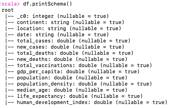
```
var datapath = "hdfs://localhost:9000/dbcovid/data/covid.csv"  
var df = spark.read.option("header", "true").option("inferSchema", "true").csv(datapath) 
```
由于考虑到csv文件包含了字段名，因此需要设置header属性为True，否则默认将第一行也会读取为记录值。而对inferSchema属性默认设置的False值，会将所有输入值均作为字符串类型进行保存，因此可以设置为True值以帮助保留浮点数的数据类型。值得注意的是，得益于Spark的处理性能，即使虚拟机仅设置了2GB内存，依然能够在一秒钟内完成创建。此时，可以通过df.printSchema()方法检查得到的数据。

三、使用Spark进行数据分析

在完成数据保存为DataFrame后，可以使用Spark对其进行数据分析。本章首先介绍数据的整体结构，然后对独立字段进行分析，最后对不同字段之间的相关性进行分析。考虑到后续可视化分析需要，此处将语句执行结果获取的数据保存为json文件，使用Spark提供的DataFrame.write.json()方法可以轻松实现。
为了便于使用Spark SQL，需要从DataFrame类型的数据上，建立临时视图：
```
df.createOrReplaceTempView("data")  
```
使用Spark SQL可以便于完成后续的操作，具体使用的分析语句见后文。对数据集进行分析得到，该数据集共有166k行记录，其中每一行对应某一个国家在特定日期的疫情情况。数据共包含六大洲、225个国家，以及不属于上述划分的部分数据如全球总数、各大洲总数。对于每一个国家而言，数据记录了最多达774天的病例情况，包括新增/总阳性病例数量，新增/总死亡数量。对于部分国家还包含了总疫苗接种剂次的记录。此外，也包含了国家的基本情况，例如人均GDP、人口、人口密度、年龄中位数、期望寿命与人类发展指数。通过这些数据及其相互联系，可以获得一个国家疫情的传播情况，并与其国家各项指标进行综合分析。
获得上述部分统计指标数值的代码如下：
```
spark.sql("select DISTINCT continent from data") -- 统计洲数量  
spark.sql("select COUNT(DISTINCT location) from data") -- 统计国家数量  
spark.sql("select COUNT(date) from data where location=='China'").show() -- 统计日期总数  
```
独立指标分析

因此，首先定义字符串数组，并在后续的实验中使用循环遍历数组中的国家/地区即可。
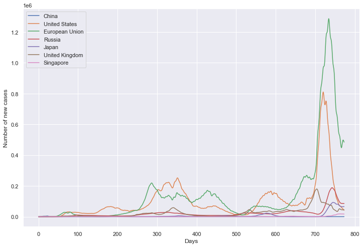
```
var locs = List("China", "United States", "European Union", "Russia", "Japan", "United Kingdom", "Singapore") 
```

（重点国家）新增病例/死亡数量

for (loc <- locs){  
spark.sql("select new_cases from data where location='"+loc+"'").write.json("/dbcovid/result/new_cases/"+loc+"/")  
spark.sql("select new_deaths from data where location='"+loc+"'").write.json("/dbcovid/result/new_deaths/"+loc+"/")  
}

（重点国家）累计病例/死亡数量

for (loc <- locs){  
spark.sql("select total_cases from data where location='"+loc+"'").write.json("/dbcovid/result/total_cases/"+loc+"/")  
spark.sql("select total_deaths from data where location='"+loc+"'").write.json("/dbcovid/result/total_deaths/"+loc+"/")  
}

（重点国家）疫苗接种剂次

for (loc <- locs){  
spark.sql("select total_vaccinations from data where location='"+loc+"'").write.json("/dbcovid/result/total_vacc/"+loc+"/")  
}

（全部国家）每百万人累计病例/死亡数量

spark.sql("select location,max(1000000*total_cases/population) from data where continent is not null group by location").write.json("/dbcovid/result/million_cases/")  
spark.sql("select location,max(1000000*total_deaths/population) from data where continent is not null group by location").write.json("/dbcovid/result/million_deaths/")

数据检查与导出

将相应的数据从HDFS导出到系统文件

bin/hdfs dfs -get /dbcovid/result ~/covid_data/

四、可视化分析

独立指标分析


import numpy as np
import pandas as pd
import matplotlib.pyplot as plt
import seaborn as sns
import json
from scipy.ndimage import gaussian_filter1d
# 定义重点国家/地区
locs = ["China", "United States", "European Union", "Russia", "Japan", "United Kingdom", "Singapore"]
# 重点国家新增病例数量
path_root = "result/new_cases/"

数据导入

all_data = []

for loc in locs:
path = path_root + loc + ".json"
tmp = pd.read_json(path, lines=True).values.squeeze() # turn to NumPy type
all_data.append(tmp)
all_data = np.array(
[
list(i) + [float("nan")] * (max([len(j) for j in all_data]) - len(i))
for i in all_data
]
)

数据 NaN 值处理

for tmp in all_data:
if np.isnan(tmp[0]):
tmp[0] = 0
for i in range(len(tmp) - 1):
if np.isnan(tmp[i + 1]):
tmp[i + 1] = tmp[i]

数据平滑

for i in range(len(all_data)):
all_data[i] = gaussian_filter1d(all_data[i], sigma=2.5)

保存为 DataFrame

df = pd.DataFrame(all_data).transpose()
df.columns = locs

绘图

plt.figure(figsize=(12, 8))
plt.xlabel('Days')
plt.ylabel('Number of new cases')
sns.lineplot(data=df, dashes=False)
plt.show()

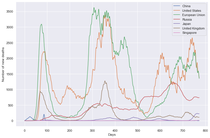
重点国家新增死亡数量

path_root = "result/new_deaths/"

all_data = []

for tmp in all_data:
if np.isnan(tmp[0]):
tmp[0] = 0
for i in range(len(tmp) - 1):
if np.isnan(tmp[i + 1]):
tmp[i + 1] = tmp[i]

for i in range(len(all_data)):
all_data[i] = gaussian_filter1d(all_data[i], sigma=2.5)

df = pd.DataFrame(all_data).transpose()
df.columns = locs

plt.figure(figsize=(12, 8))
plt.xlabel('Days')
plt.ylabel('Number of new deaths')
sns.lineplot(data=df, dashes=False)
plt.show()

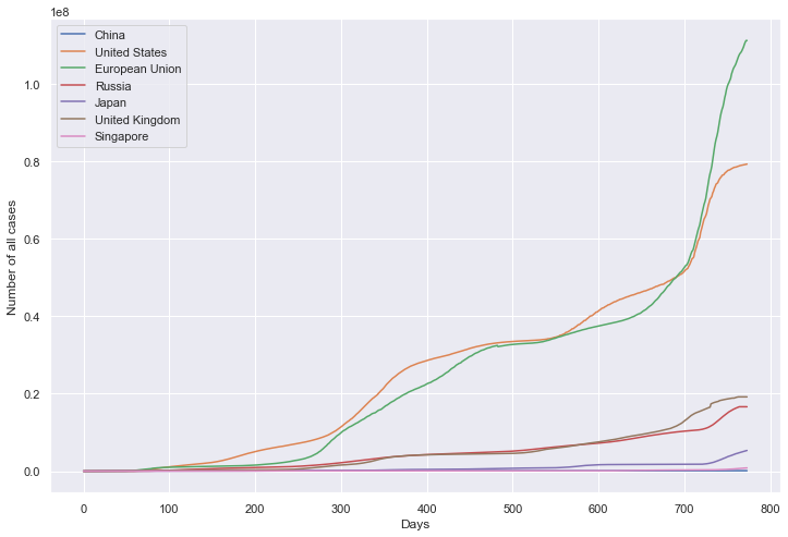
重点国家累计病例数量

path_root = "result/total_cases/"

数据导入

all_data = []

for loc in locs:
path = path_root + loc + ".json"
tmp = pd.read_json(path, lines=True).values.squeeze() # NumPy type
all_data.append(tmp)
all_data = np.array(
[
list(i) + [float("nan")] * (max([len(j) for j in all_data]) - len(i))
for i in all_data
]
)

数据 NaN 值处理

for tmp in all_data:
if np.isnan(tmp[0]):
tmp[0] = 0
for i in range(len(tmp) - 1):
if np.isnan(tmp[i + 1]):
tmp[i + 1] = tmp[i]

本数据不使用平滑。

保存为 DataFrame

df = pd.DataFrame(all_data).transpose()
df.columns = locs

绘图

plt.figure(figsize=(12, 8))
plt.xlabel('Days')
plt.ylabel('Number of all cases')
sns.lineplot(data=df, dashes=False)
plt.show()

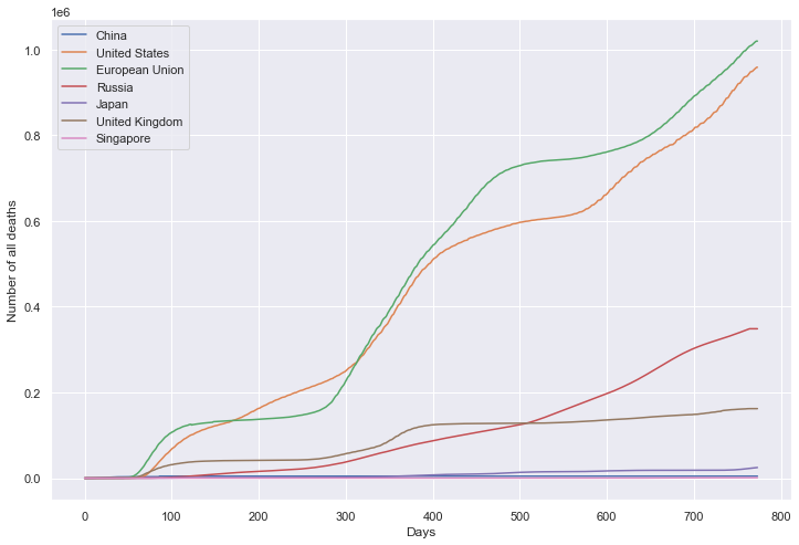
重点国家累计死亡数量

path_root = "result/total_deaths/"

数据导入

all_data = []

数据 NaN 值处理

for tmp in all_data:
if np.isnan(tmp[0]):
tmp[0] = 0
for i in range(len(tmp) - 1):
if np.isnan(tmp[i + 1]):
tmp[i + 1] = tmp[i]

本数据不使用平滑。

保存为 DataFrame

df = pd.DataFrame(all_data).transpose()
df.columns = locs

绘图

plt.figure(figsize=(12, 8))
plt.xlabel('Days')
plt.ylabel('Number of all deaths')
sns.lineplot(data=df, dashes=False)
plt.show()

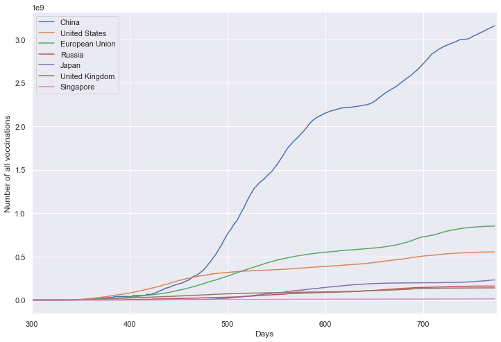
重点国家累计疫苗接种剂次

path_root = "result/total_vacc/"

数据导入

all_data = []

数据 NaN 值处理

for tmp in all_data:
if np.isnan(tmp[0]):
tmp[0] = 0
for i in range(len(tmp) - 1):
if np.isnan(tmp[i + 1]):
tmp[i + 1] = tmp[i]

本数据不使用平滑。

保存为 DataFrame

df = pd.DataFrame(all_data).transpose()
df.columns = locs

绘图

plt.figure(figsize=(12, 8))
plt.xlabel('Days')
plt.ylabel('Number of all voccinations')
fig = sns.lineplot(data=df, dashes=False)
fig.set_xlim(300, 775)
plt.show()

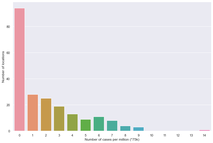
全部国家每百万人累计病例

读取文件

path = "result/million_cases.json"
all_data = pd.read_json(path, lines=True)
all_data.columns = ['location', 'data']
tmp_data = pd.DataFrame(all_data, columns=['data']).values.squeeze() # NumPy type

处理 NaN 缺失值

number_data = [x for x in tmp_data if not np.isnan(x)]

保存密度数据

countdata = [0 for in range(15)]
for i in number_data:
count_data[int(i/5e4)] += 1

保存为 DataFrame

df = pd.DataFrame(count_data).transpose()

绘图

plt.figure(figsize=(12, 8))
sns.barplot(data=df)
plt.xlabel('Number of cases per million (*75k)')
plt.ylabel('Number of locations')
plt.show()

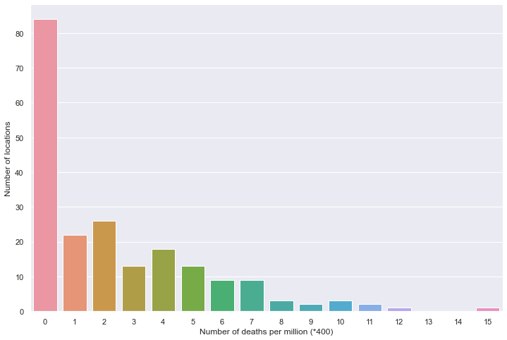
全部国家每百万人累计死亡

读取文件

path = "result/million_deaths.json"
all_data = pd.read_json(path, lines=True)
all_data.columns = ['location', 'data']
tmp_data = pd.DataFrame(all_data, columns=['data']).values.squeeze() # NumPy type

处理 NaN 缺失值

number_data = [x for x in tmp_data if not np.isnan(x)]

保存密度数据

countdata = [0 for in range(16)]
for i in number_data:
count_data[int(i/400)] += 1

保存为 DataFrame

df = pd.DataFrame(count_data).transpose()

绘图

plt.figure(figsize=(12, 8))
sns.barplot(data=df)
plt.xlabel('Number of deaths per million (*400)')
plt.ylabel('Number of locations')
plt.show()

新增病例数量
![](https://dblab.xmu.edu.cn/blog/wp-content/uploads/2022/09/新增病例数量.png)
新增死亡数量
![](https://dblab.xmu.edu.cn/blog/wp-content/uploads/2022/09/新增死亡数量.png)
累计病例数量
![](https://dblab.xmu.edu.cn/blog/wp-content/uploads/2022/09/累计病例数量.png)
累计死亡数量
![](https://dblab.xmu.edu.cn/blog/wp-content/uploads/2022/09/累计死亡数量.png)
累计疫苗数量
![](https://dblab.xmu.edu.cn/blog/wp-content/uploads/2022/09/累计疫苗数量.png)
百万人累计病例
![](https://dblab.xmu.edu.cn/blog/wp-content/uploads/2022/09/百万人累计病例.png)
百万人累计死亡
![](https://dblab.xmu.edu.cn/blog/wp-content/uploads/2022/09/百万人累计死亡.png)
### 相关性分析
```python
import numpy as np
import pandas as pd
import matplotlib.pyplot as plt
import seaborn as sns
import json
from scipy.ndimage import gaussian_filter1d

sns.set_style("darkgrid")
# 定义重点国家/地区
locs = ["China", "United States", "European Union", "Russia", "Japan", "United Kingdom", "Singapore"]

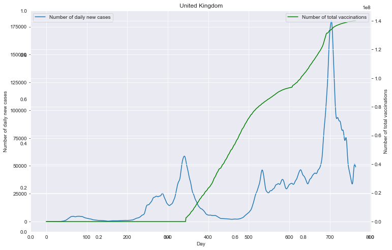
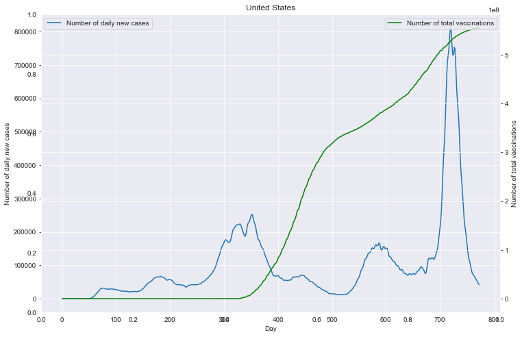
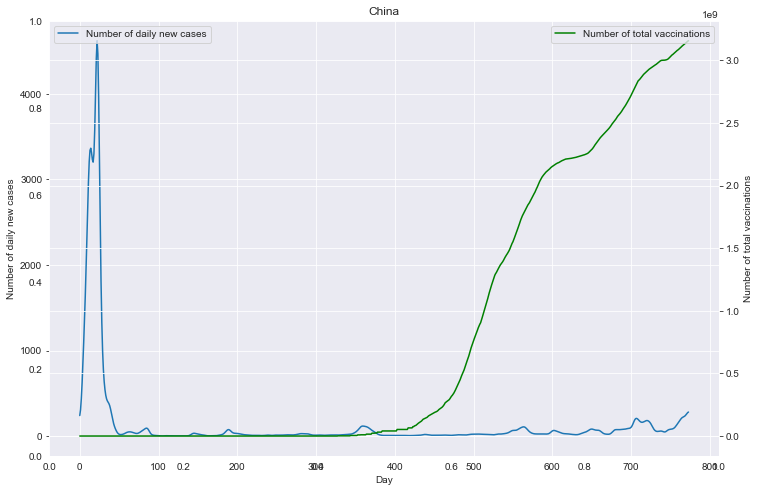
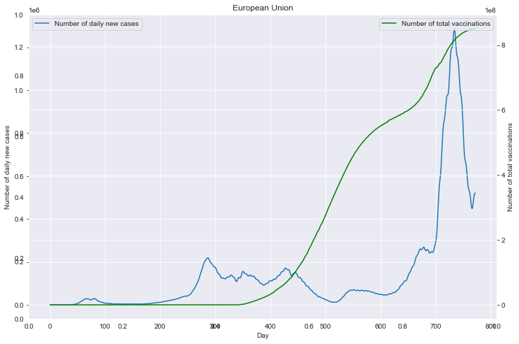
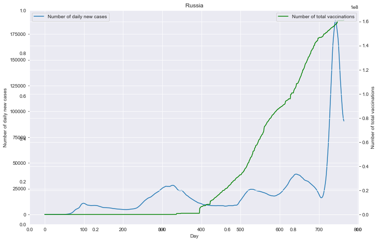
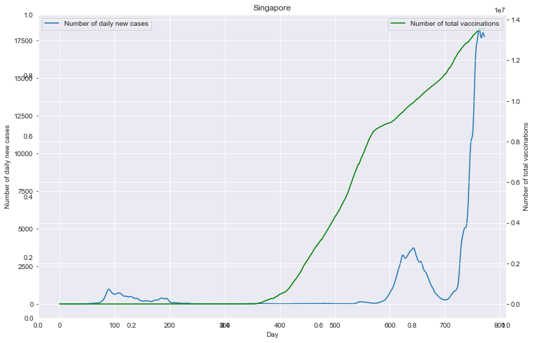
# 重点国家新增病例数量与疫苗剂次关系
path_root = "result/cases_with_vaccs/"

# 各国家独立保存图像
for loc in locs:
    path = path_root + loc + ".json"
    data = pd.read_json(path, lines=True).values.squeeze()  # turn to NumPy type
    data = np.array(data).T

    # 数据 NaN 值处理
    for tmp in data:
        if np.isnan(tmp[0]):
            tmp[0] = 0
        for i in range(len(tmp) - 1):
            if np.isnan(tmp[i + 1]):
                tmp[i + 1] = tmp[i]

    # 数据平滑
    data[0] = gaussian_filter1d(data[0], sigma=2.5)

    # 保存 DataFrame
    df0 = pd.DataFrame(data[0])
    df0.columns = ['Number of daily new cases']
    df1 = pd.DataFrame(data[1])
    df1.columns = ['Number of total vaccinations']

    # 绘图
    fig = plt.figure(figsize=(12, 8))
    plt.title(loc)
    ax1 = fig.add_subplot(111)
    df0.plot(ax=ax1, style='-')
    plt.xlabel('Day')
    ax1.set_ylabel('Number of daily new cases')
    # ax1.set_yticks(np.arange(0, 1.5e6, 1e5))
    plt.legend(loc=2) # 10

    ax2 = ax1.twinx()
    df1.plot(ax=ax2, style='-', color='green')
    ax2.set_ylabel('Number of total vaccinations')
    # ax2.set_yticks(np.arange(0, 3.5e9, 5e8))
    plt.legend(loc=1) # 10

    plt.savefig(u'新增与疫苗关系_'+loc+'.png', bbox_inches='tight')

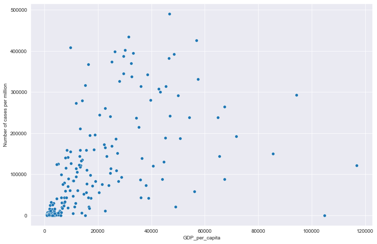
# 全部国家每百万人累计病例&人均GDP关系

# 读取文件
path = "result/million_cases_with_gdp.json"
all_data = pd.read_json(path, lines=True)
all_data.columns = ['location', 'data', 'gdp']

all_data.dropna(inplace=True)

# 绘图
plt.figure(figsize=(12, 8))
sns.scatterplot(data=all_data, x='gdp', y='data')
plt.xlabel('GDP_per_capita')
plt.ylabel('Number of cases per million')
plt.show()

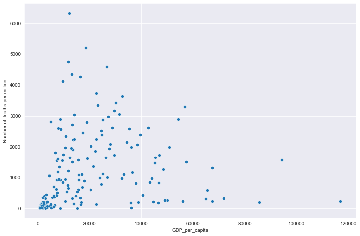
# 全部国家每百万人累计死亡&人均GDP关系

# 读取文件
path = "result/million_deaths_with_gdp.json"
all_data = pd.read_json(path, lines=True)
all_data.columns = ['location', 'data', 'gdp']

all_data.dropna(inplace=True)

# 绘图
plt.figure(figsize=(12, 8))
sns.scatterplot(data=all_data, x='gdp', y='data')
plt.xlabel('GDP_per_capita')
plt.ylabel('Number of deaths per million')
plt.show()

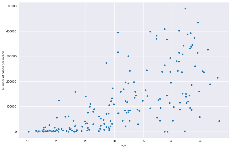
# 全部国家每百万人累计病例&年龄中位数关系

# 读取文件
path = "result/million_cases_with_age.json"
all_data = pd.read_json(path, lines=True)
all_data.columns = ['location', 'data', 'age']

all_data.dropna(inplace=True)

# 绘图
plt.figure(figsize=(12, 8))
sns.scatterplot(data=all_data, x='age', y='data')
plt.xlabel('age')
plt.ylabel('Number of cases per million')
plt.show()

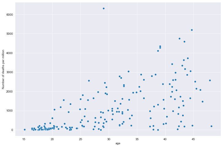
# 全部国家每百万人累计死亡&年龄中位数关系

# 读取文件
path = "result/million_deaths_with_age.json"
all_data = pd.read_json(path, lines=True)
all_data.columns = ['location', 'data', 'age']

all_data.dropna(inplace=True)

# 绘图
plt.figure(figsize=(12, 8))
sns.scatterplot(data=all_data, x='age', y='data')
plt.xlabel('age')
plt.ylabel('Number of deaths per million')
plt.show()

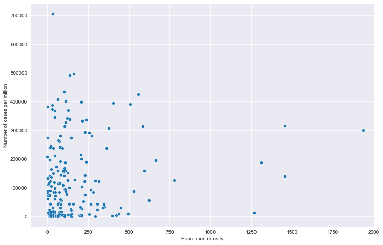
# 全部国家每百万人累计病例&人口密度关系

# 读取文件
path = "result/million_cases_with_density.json"
all_data = pd.read_json(path, lines=True)
all_data.columns = ['location', 'data', 'den']

all_data.dropna(inplace=True)

# 绘图
plt.figure(figsize=(12, 8))
fig = sns.scatterplot(data=all_data, x='den', y='data')
# fig.set_xticks(np.arange(0,5000,250))
fig.set_xlim(-100, 2000)
plt.xlabel('Population density')
plt.ylabel('Number of cases per million')
plt.show()

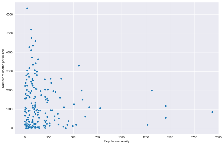
# 全部国家每百万人累计死亡&人口密度关系

# 读取文件
path = "result/million_deaths_with_density.json"
all_data = pd.read_json(path, lines=True)
all_data.columns = ['location', 'data', 'den']

all_data.dropna(inplace=True)

# 绘图
plt.figure(figsize=(12, 8))
fig = sns.scatterplot(data=all_data, x='den', y='data')
# fig.set_xticks(np.arange(0,5000,250))
fig.set_xlim(-100, 2000)
plt.xlabel('Population density')
plt.ylabel('Number of deaths per million')
plt.show()

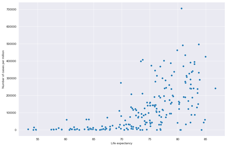
# 全部国家每百万人累计病例&期望寿命关系

# 读取文件
path = "result/million_cases_with_lifeexp.json"
all_data = pd.read_json(path, lines=True)
all_data.columns = ['location', 'data', 'exp']

all_data.dropna(inplace=True)

# 绘图
plt.figure(figsize=(12, 8))
fig = sns.scatterplot(data=all_data, x='exp', y='data')
plt.xlabel('Life expectancy')
plt.ylabel('Number of cases per million')
plt.show()

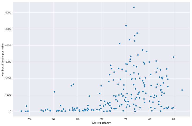
# 全部国家每百万人累计死亡&期望寿命关系

# 读取文件
path = "result/million_deaths_with_lifeexp.json"
all_data = pd.read_json(path, lines=True)
all_data.columns = ['location', 'data', 'exp']

all_data.dropna(inplace=True)

# 绘图
plt.figure(figsize=(12, 8))
fig = sns.scatterplot(data=all_data, x='exp', y='data')
plt.xlabel('Life expectancy')
plt.ylabel('Number of deaths per million')
plt.show()

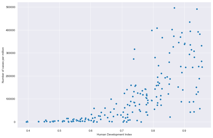
# 全部国家每百万人累计病例&hdi关系

# 读取文件
path = "result/million_cases_with_hdi.json"
all_data = pd.read_json(path, lines=True)
all_data.columns = ['location', 'data', 'hdi']

all_data.dropna(inplace=True)

# 绘图
plt.figure(figsize=(12, 8))
fig = sns.scatterplot(data=all_data, x='hdi', y='data')
plt.xlabel('Human Development Index')
plt.ylabel('Number of cases per million')
plt.show()

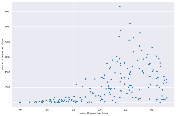
# 全部国家每百万人累计死亡&hdi关系

# 读取文件
path = "result/million_deaths_with_hdi.json"
all_data = pd.read_json(path, lines=True)
all_data.columns = ['location', 'data', 'hdi']

all_data.dropna(inplace=True)

# 绘图
plt.figure(figsize=(12, 8))
fig = sns.scatterplot(data=all_data, x='hdi', y='data')
plt.xlabel('Human Development Index')
plt.ylabel('Number of deaths per million')
plt.show()

重点国家新增病例数量与疫苗剂次关系

全部国家每百万人累计病例&人均GDP关系

全部国家每百万人累计死亡&人均GDP关系

全部国家每百万人累计病例&年龄中位数关系

全部国家每百万人累计死亡&年龄中位数关系

全部国家每百万人累计病例&人口密度关系

全部国家每百万人累计死亡&人口密度关系

全部国家每百万人累计病例&期望寿命关系

全部国家每百万人累计死亡&期望寿命关系

全部国家每百万人累计病例&hdi关系

全部国家每百万人累计死亡&hdi关系