
【版权声明】版权所有,严禁转载,严禁用于商业用途,侵权必究。
作者:厦门大学 2021级研究生 徐常升
指导老师:厦门大学数据库实验室 林子雨 博士/副教授
相关教材:林子雨、郑海山、赖永炫编著《Spark编程基础(Scala版)》
【查看基于Scala语言的Spark数据分析案例集锦】
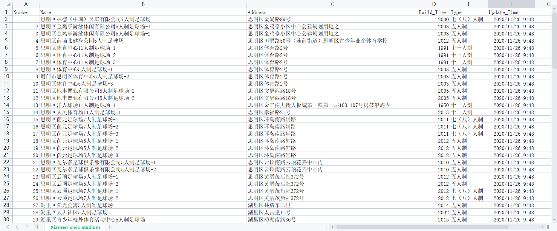
本案例的数据集来自厦门市大数据安全开放平台(厦门市大数据安全开放平台)中的数据集:厦门市市民球场信息数据,以scala为编程语言,使用大数据框架Spark对数据进行处理分析,并对分析结果进行可视化。
一、实验环境:
我将使用以下实验环境来进行实验。
1.Linux:Ubuntu 18.04.6 LTS
2.Hadoop:3.1.3
3.Spark:3.2.0
4.python:3.8.10
5.Scala:2.12.15
6.sbt:1.6.2
7.IDEA 22.1
8.VMware workstation 16 pro
9.pyecharts 1.9.1
二、环境搭建:
1.安装Linux操作系统:在VMware上安装Ubuntu 20.04.3 LTS;
2.安装Hadoop:需要在Linux系统上安装Hadoop3.1.3;
3.安装Spark:需要在Linux系统上安装Spark3.2.0;
三、数据集:
1.数据集的下载
本次实验数据集来自厦门市大数据安全开放平台中的数据,以数据集Xiamen_civic_stadium.csv为分析主体。可以从百度网盘下载数据集(提取码:ziyu)。
每个数据包含以下字段:
字段名称 字段含义 例子
(1)Number 作为主键标识 1,2,3,...
(2)Name 球场名称 **足球场,...
(3)Address 球场地址 区路**号,...
(4)Build_Time 建成时间 2009,...
(5)Type 球场类型 七(八)人制,五人制,...
(6)Update_Time 信息更新时间 2020/11/26 9:48,...
2.数据集上传HDFS
为了更方便的对 csv 文件进行处理,将处理好的文件 Xiamen_civic_stadium.csv 存储到 HDFS 上方便进一步的处理,使用下面命令将文件上传至 HDFS:
/usr/local/hadoop/sbin/start-dfs.sh
hdfs dfs -put /home/hadoop/Bigdata/XCS/Xiamen_civic_stadium.csv
四、使用 Spark 进行数据分析
1.调用csv文件从HDFS上
//download file from HDFS
val filepath="hdfs://localhost:9000/user/hadoop/Xiamen_civic_stadium.csv"
2.通过地址地段(Address)对球场分布进行分析
// Analysis 1 : Address
  def main(args: Array[String]): Unit = {
    // read the csv
    val df=spark.read.options(
      Map("inferSchema"->"true","delimiter"->",","header"->"true")).csv(filepath)

    // select the file Siming District and Count the number of Siming District
    df.createOrReplaceTempView("Siming")
    val Siming = spark.sql("select * from Siming where `Address` like '%思明区%'")
    val Siming_count = spark.sql("select * from Siming where `Address` like '%思明区%'").count
    // Siming.show()
    Siming.write.option("header",value = true).mode("overwrite").csv("file:///home/hadoop/IdeaProjects/work/Result_Address/Siming_District.csv")

    // select the file Huli District and Count the number of Huli District
    df.createOrReplaceTempView("Huli")
    val Huli = spark.sql("select * from Huli where `Address` like '%湖里区%'")
    val Huli_count = spark.sql("select * from Huli where `Address` like '%湖里区%'").count()
    Huli.write.option("header",value = true).mode("overwrite").csv("file:///home/hadoop/IdeaProjects/work/Result_Address/Huli_District.csv")

    // select the file Jimei District and Count the number of Jimei District
    df.createOrReplaceTempView("Jimei")
    val Jimei = spark.sql("select * from Jimei where `Address` like '%集美区%'")
    val Jimei_count = spark.sql("select * from Jimei where `Address` like '%集美区%'").count()
    Jimei.write.option("header",value = true).mode("overwrite").csv("file:///home/hadoop/IdeaProjects/work/Result_Address/Jimei_District.csv")

    // select the file Haicang District and Count the number of Haicang District
    df.createOrReplaceTempView("Haicang")
    val Haicang = spark.sql("select * from Haicang where `Address` like '%海沧区%'")
    val Haicang_count = spark.sql("select * from Haicang where `Address` like '%海沧区%'").count()
    Haicang.write.option("header",value = true).mode("overwrite").csv("file:///home/hadoop/IdeaProjects/work/Result_Address/Haicang_District.csv")

    // select the file Tongan District and Count the number of Tongan District
    df.createOrReplaceTempView("Tongan")
        val Tongan = spark.sql("select * from Tongan where `Address` like '%同安区%'")
    val Tongan_count = spark.sql("select * from Tongan where `Address` like '%同安区%'").count()
    Tongan.write.option("header",value = true).mode("overwrite").csv("file:///home/hadoop/IdeaProjects/work/Result_Address/Tongan_District.csv")

    // select the file Xiangan District and Count the number of Xiangan District
    df.createOrReplaceTempView("Xiangan")
    val Xiangan = spark.sql("select * from Xiangan where `Address` like '%翔安区%'")
    val Xiangan_count = spark.sql("select * from Xiangan where `Address` like '%翔安区%'").count()
    Xiangan.write.option("header",value = true).mode("overwrite").csv("file:///home/hadoop/IdeaProjects/work/Result_Address/Xiangan_District.csv")
3.地址(Address)与球场数量(Count)的关系
// Rank the total number of different regions in descending order
    // use createDataFrame to create DataFrame
    val Sum = spark.createDataFrame(Seq(
      ("思明区", Siming_count),
      ("湖里区", Huli_count),
      ("集美区", Jimei_count),
      ("海沧区", Haicang_count),
      ("同安区", Tongan_count),
      ("翔安区", Xiangan_count),
    )).toDF("Add_simple", "Count")   Sum.write.option("header",value=true).mode("overwrite").csv("file:///home/hadoop/IdeaProjects/work/Result_Address/Sum.csv")
4.通过球场建造时间(BuildTime)对球场分布进行分析
// select the information according to the different eras
    // before 1999.12.31
    df.createOrReplaceTempView("BuildTime")
    val BuildTime1 = spark.sql("select * from BuildTime where Build_Time <2000 order by Build_Time desc")
    BuildTime1.write.option("header",value = true).mode("overwrite").csv("file:///home/hadoop/IdeaProjects/work/Result_BuildTime/BuildTime_before_2000.csv")
    // 2000.1.1 - 2009.12.31
    df.createOrReplaceTempView("BuildTime")
    val BuildTime2 = spark.sql("select * from BuildTime where Build_Time >= 2000 and Build_Time < 2010 order by Build_Time desc")
    BuildTime2.write.option("header",value = true).mode("overwrite").csv("file:///home/hadoop/IdeaProjects/work/Result_BuildTime/BuildTime_2000_2009.csv")
    // 2010.1.1 - 2019.12.31
    df.createOrReplaceTempView("BuildTime")
    val BuildTime3 = spark.sql("select * from BuildTime where Build_Time >= 2010 and Build_Time < 2020 order by Build_Time desc")
    BuildTime3.write.option("header",value = true).mode("overwrite").csv("file:///home/hadoop/IdeaProjects/work/Result_BuildTime/BuildTime2010_2019.csv")
    // 2020.1.1 - Today
    df.createOrReplaceTempView("BuildTime")
    val BuildTime4 = spark.sql("select * from BuildTime where Build_Time >= 2020 order by Build_Time desc")
    BuildTime4.write.option("header",value = true).mode("overwrite").csv("file:///home/hadoop/IdeaProjects/work/Result_BuildTime/BuildTime_2020_Today.csv")
5.建造时间(BuildTime)与球场数量(Count)的关系
// select the all build time
df.createOrReplaceTempView("BuildTime")
// Sort as Time
val BuildTime_SortTime = spark.sql("select Build_Time, count(*) as Count from BuildTime GROUP BY Build_Time order by Build_Time desc")
// Sort as Count
    val BuildTime_SortCount = spark.sql("select Build_Time, count(*) as Count from BuildTime GROUP BY Build_Time order by count(*) desc")
    val Time_Sum = spark.sql("select Build_Time, count(*) as Count from BuildTime GROUP BY Build_Time order by count(*) desc").count()
    println(Time_Sum)
    // BuildTime_SortCount.show()
    BuildTime_SortTime.write.option("header",value = true).mode("overwrite").csv("file:///home/hadoop/IdeaProjects/work/Result_BuildTime/CountTime_SortTime.csv")
BuildTime_SortCount.write.option("header",value = true).mode("overwrite").csv("file:///home/hadoop/IdeaProjects/work/Result_BuildTime/CountTime_SortCount.csv")
6.选择不同区中建造时间(BuildTime)与球场数量(Count)的关系
// Different district relationship between count and time
    val filepath1="hdfs://localhost:9000/user/hadoop/Haicang_District.csv"
    val filepath2="hdfs://localhost:9000/user/hadoop/Huli_District.csv"
    val filepath3="hdfs://localhost:9000/user/hadoop/Jimei_District.csv"
    val filepath4="hdfs://localhost:9000/user/hadoop/Siming_District.csv"
    val filepath5="hdfs://localhost:9000/user/hadoop/Tongan_District.csv"
    val filepath6="hdfs://localhost:9000/user/hadoop/Xiangan_District.csv"

    val df1=spark.read.options(
      Map("inferSchema"->"true","delimiter"->",","header"->"true")).csv(filepath1)
    val df2=spark.read.options(
      Map("inferSchema"->"true","delimiter"->",","header"->"true")).csv(filepath2)
    val df3=spark.read.options(
      Map("inferSchema"->"true","delimiter"->",","header"->"true")).csv(filepath3)
    val df4=spark.read.options(
      Map("inferSchema"->"true","delimiter"->",","header"->"true")).csv(filepath4)
    val df5=spark.read.options(
      Map("inferSchema"->"true","delimiter"->",","header"->"true")).csv(filepath5)
    val df6=spark.read.options(
      Map("inferSchema"->"true","delimiter"->",","header"->"true")).csv(filepath6)
    // select the district build time and count
    df1.createOrReplaceTempView("Haicang")
    // Sort as Time
    val Haicang = spark.sql("select Build_Time, count(*) as Count from Haicang GROUP BY Build_Time order by Build_Time desc")
    Haicang.write.option("header",value = true).mode("overwrite").csv("file:///home/hadoop/IdeaProjects/work/Result_BuildTime/Haicang.csv")

    df2.createOrReplaceTempView("Huli")
    // Sort as Time
    val Huli = spark.sql("select Build_Time, count(*) as Count from Huli GROUP BY Build_Time order by Build_Time desc")
    Huli.write.option("header",value = true).mode("overwrite").csv("file:///home/hadoop/IdeaProjects/work/Result_BuildTime/Huli.csv")

    df3.createOrReplaceTempView("Jimei")
    // Sort as Time
    val Jimei = spark.sql("select Build_Time, count(*) as Count from Jimei GROUP BY Build_Time order by Build_Time desc")
    Jimei.write.option("header",value = true).mode("overwrite").csv("file:///home/hadoop/IdeaProjects/work/Result_BuildTime/Jimei.csv")
        df4.createOrReplaceTempView("Siming")
    // Sort as Time
    val Siming = spark.sql("select Build_Time, count(*) as Count from Siming GROUP BY Build_Time order by Build_Time desc")
    Siming.write.option("header",value = true).mode("overwrite").csv("file:///home/hadoop/IdeaProjects/work/Result_BuildTime/Siming.csv")

    df5.createOrReplaceTempView("Tongan")
    // Sort as Time
    val Tongan = spark.sql("select Build_Time, count(*) as Count from Tongan GROUP BY Build_Time order by Build_Time desc")
    Tongan.write.option("header",value = true).mode("overwrite").csv("file:///home/hadoop/IdeaProjects/work/Result_BuildTime/Tongan.csv")

    df6.createOrReplaceTempView("Xiangan")
    // Sort as Time
    val Xiangan = spark.sql("select Build_Time, count(*) as Count from Xiangan GROUP BY Build_Time order by Build_Time desc")
    Xiangan.write.option("header",value = true).mode("overwrite").csv("file:///home/hadoop/IdeaProjects/work/Result_BuildTime/Xiangan.csv")
7.通过球场类型(Type)对球场分布进行分析
// select the information according to the different types
    // 五人制
    df.createOrReplaceTempView("Five")
    val BuildTime1 = spark.sql("select * from Five where Type = '五人制' order by Build_Time desc")
    BuildTime1.write.option("header",value = true).mode("overwrite").csv("file:///home/hadoop/IdeaProjects/work/Result_Type/Five.csv)
    // 七(八)人制
    df.createOrReplaceTempView("Seven")
    val BuildTime2 = spark.sql("select * from Seven where Type = '七(八)人制' order by Build_Time desc")
    BuildTime2.write.option("header",value = true).mode("overwrite").csv("file:///home/hadoop/IdeaProjects/work/Result_Type/Seven.csv")
    // 十一人制
    df.createOrReplaceTempView("Eleven")
    val BuildTime3 = spark.sql("select * from Eleven where Type = '十一人制' order by Build_Time desc")
    BuildTime3.write.option("header",value = true).mode("overwrite").csv("file:///home/hadoop/IdeaProjects/work/Result_Type/Eleven.csv")
8.球场类型(Type)与球场数量(Count)的关系
// select the all Course type
    df.createOrReplaceTempView("Type")
    val Type_SortCount = spark.sql("select Type, count(*) as Count from Type GROUP BY Type order by count(*) desc")
    val Type_Sum = spark.sql("select Type, count(*) as Count from Type GROUP BY Type order by count(*) desc").count()
    println(Type_Sum)
    // Type_SortCount.show()
    Type_SortCount.write.option("header",value = true).mode("overwrite").csv("file:///home/hadoop/IdeaProjects/work/Result_Type/Type_SortCount.csv")
9.不同区球场类型(Type)与球场数量(Count)的关系
// Different district relationship between count and type
    val filepath1="hdfs://localhost:9000/user/hadoop/Haicang_District.csv"
    val filepath2="hdfs://localhost:9000/user/hadoop/Huli_District.csv"
    val filepath3="hdfs://localhost:9000/user/hadoop/Jimei_District.csv"
    val filepath4="hdfs://localhost:9000/user/hadoop/Siming_District.csv"
    val filepath5="hdfs://localhost:9000/user/hadoop/Tongan_District.csv"
    val filepath6="hdfs://localhost:9000/user/hadoop/Xiangan_District.csv"

    val df1=spark.read.options(
      Map("inferSchema"->"true","delimiter"->",","header"->"true")).csv(filepath1)
    val df2=spark.read.options(
      Map("inferSchema"->"true","delimiter"->",","header"->"true")).csv(filepath2)
    val df3=spark.read.options(
      Map("inferSchema"->"true","delimiter"->",","header"->"true")).csv(filepath3)
    val df4=spark.read.options(
      Map("inferSchema"->"true","delimiter"->",","header"->"true")).csv(filepath4)
    val df5=spark.read.options(
      Map("inferSchema"->"true","delimiter"->",","header"->"true")).csv(filepath5)
    val df6=spark.read.options(
      Map("inferSchema"->"true","delimiter"->",","header"->"true")).csv(filepath6)
    // select the district type and count
    df1.createOrReplaceTempView("Haicang")
    // Sort as type
    val Haicang = spark.sql("select Type, count(*) as Count from Haicang GROUP BY Type order by Type")
    Haicang.write.option("header",value = true).mode("overwrite").csv("file:///home/hadoop/IdeaProjects/work/Result_Type/Haicang_Type.csv")
    df2.createOrReplaceTempView("Huli")
    // Sort as type
    val Huli = spark.sql("select Type, count(*) as Count from Huli GROUP BY Type order by Type")
    Huli.write.option("header",value = true).mode("overwrite").csv("file:///home/hadoop/IdeaProjects/work/Result_Type/Huli_Type.csv")

    df3.createOrReplaceTempView("Jimei")
    // Sort as type
    val Jimei = spark.sql("select Type, count(*) as Count from Jimei GROUP BY Type order by Type")
    Jimei.write.option("header",value = true).mode("overwrite").csv("file:///home/hadoop/IdeaProjects/work/Result_Type/Jimei_Type.csv")

    df4.createOrReplaceTempView("Siming")
    // Sort as type
    val Siming = spark.sql("select Type, count(*) as Count from Siming GROUP BY Type order by Type")
    Siming.write.option("header",value = true).mode("overwrite").csv("file:///home/hadoop/IdeaProjects/work/Result_BuildTime/Siming_Type.csv")

    df5.createOrReplaceTempView("Tongan")
    // Sort as type
    val Tongan = spark.sql("select Type, count(*) as Count from Tongan GROUP BY Type order by Type")
    Tongan.write.option("header",value = true).mode("overwrite").csv("file:///home/hadoop/IdeaProjects/work/Result_BuildTime/Tongan_Type.csv")

    df6.createOrReplaceTempView("Xiangan")
    // Sort as type
    val Xiangan = spark.sql("select Type, count(*) as Count from Xiangan GROUP BY Type order by Type")
    Xiangan.write.option("header",value = true).mode("overwrite").csv("file:///home/hadoop/IdeaProjects/work/Result_BuildTime/Xiangan_Type.csv")
10.不同类型(Type)球场数量(Count)与建造时间(BuildTime)的关系
// Different type relationship between count and time
    val filepath7="hdfs://localhost:9000/user/hadoop/Eleven.csv"
    val filepath8="hdfs://localhost:9000/user/hadoop/Five.csv"
    val filepath9="hdfs://localhost:9000/user/hadoop/Seven.csv"
    val df7=spark.read.options(
      Map("inferSchema"->"true","delimiter"->",","header"->"true")).csv(filepath7)
    val df8=spark.read.options(
      Map("inferSchema"->"true","delimiter"->",","header"->"true")).csv(filepath8)
    val df9=spark.read.options(
      Map("inferSchema"->"true","delimiter"->",","header"->"true")).csv(filepath9)
    // select the district buildtime and count
    df1.createOrReplaceTempView("Eleven")
    // Sort as Time
    val Eleven = spark.sql("select Build_Time, count(*) as Count from Eleven GROUP BY Build_Time order by Build_Time desc")
    Eleven.write.option("header",value = true).mode("overwrite").csv("file:///home/hadoop/IdeaProjects/work/Result_Type/Eleven_time.csv")
    df2.createOrReplaceTempView("Five")
    // Sort as Time
    val Five = spark.sql("select Build_Time, count(*) as Count from Five GROUP BY Build_Time order by Build_Time desc")
    Five.write.option("header",value = true).mode("overwrite").csv("file:///home/hadoop/IdeaProjects/work/Result_Type/Five_time.csv")
    df3.createOrReplaceTempView("Seven")
    // Sort as Time
    val Seven = spark.sql("select Build_Time, count(*) as Count from Seven GROUP BY Build_Time order by Build_Time desc")
    Seven.write.option("header",value = true).mode("overwrite").csv("file:///home/hadoop/IdeaProjects/work/Result_Type/Seven_time.csv")
五、可视化
为了支持Python可视化分析,还需要执行如下命令安装pandas,pyecharts组件:
sudo apt-get install python3-pip
pip3 install pandas
pip3 install pyecharts
1.厦门市球场分布图_Map
import pandas as pd
from pyecharts.charts import Map
from pyecharts import options as opts
file = pd.read_csv('Sum.csv')
df = pd.DataFrame(file)
data = []
for i in range(len(df)):
    document = df[i:i + 1]
    Add_simple = document['Add_simple'][i]
    Count = document['Count'][i]
    data.append((Add_simple, str(Count)))
Map_xiamen = (
    Map(init_opts=opts.InitOpts(width="1000px", height="600px"))
        .add('厦门市', data, maptype='厦门')
        .set_global_opts(
        title_opts=opts.TitleOpts(title="球场信息分布", pos_right="center", pos_top="5%"),
        visualmap_opts=opts.VisualMapOpts(max_=40))
        .set_series_opts(label_opts=opts.LabelOpts(is_show=False))
        .render("Xiamen.html"))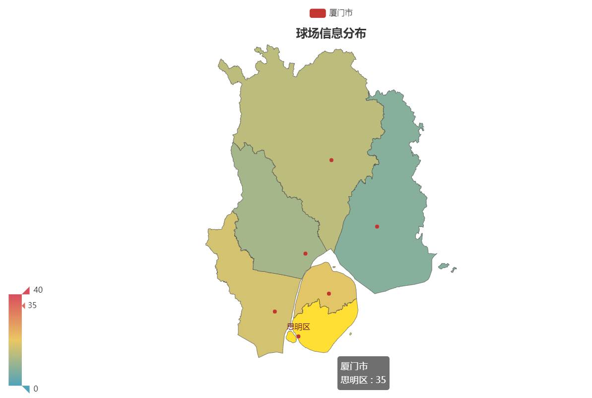
2.厦门市球场分布图 Bar
from pyecharts.charts import Bar
import pandas as pd
from pyecharts import options as opts

file = pd.read_csv('Sum.csv')
df = pd.DataFrame(file)
columns = []
data = []
for i in range(len(df)):
    document = df[i:i + 1]
    Add_simple = document['Add_simple'][i]
    Count = document['Count'][i]
    columns.append(Add_simple)
    data.append(str(Count))
bar = (
    Bar()
    .add_xaxis(columns)
    .add_yaxis("球场数量", data)
    .set_global_opts(title_opts=opts.TitleOpts(title="不同区域的球场分布数量"))
    .render("Xiamen_bar.html")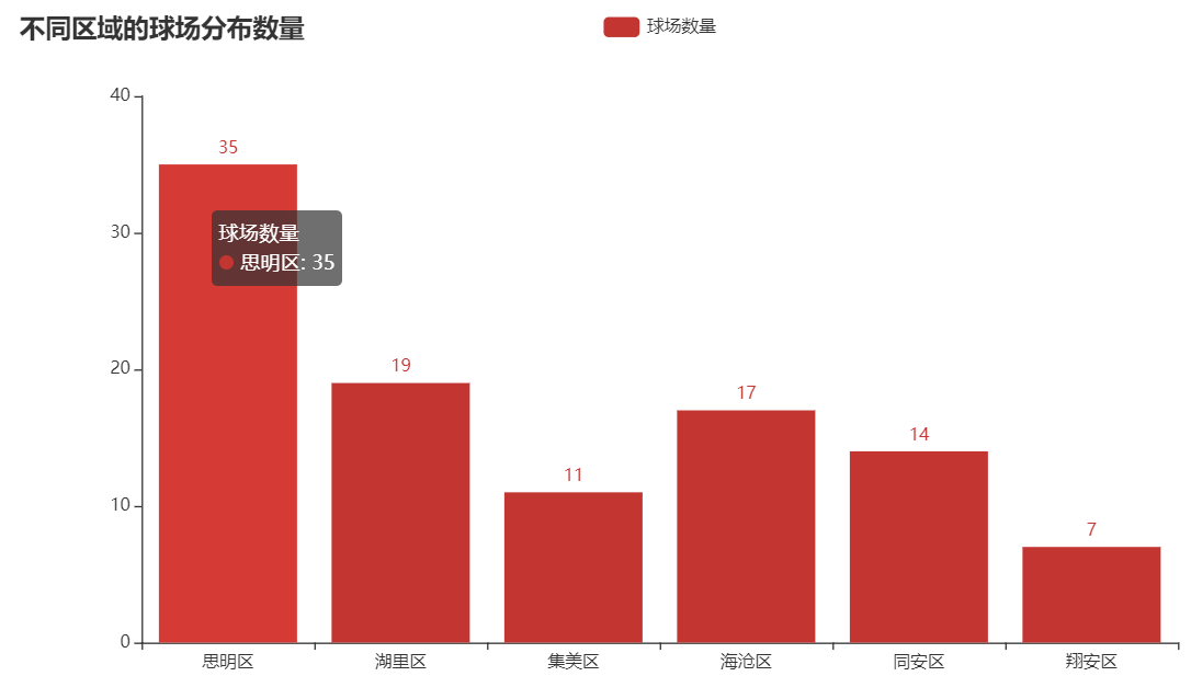
由图中可以得知思明区的球场数量最多,翔安区的球场数量最少。
3.厦门市球场建造数量(Count)与建造时间(BuildTime)的关系
from pyecharts.charts import Line
import pandas as pd
from pyecharts import options as opts
file = pd.read_csv('CountTime_SortTime.csv')
df = pd.DataFrame(file)
columns = []
data = []
for i in range(len(df)-1, -1, -1):
    document = df[i:i + 1]
    Build_Time = document['Build_Time'][i]
    Count = document['Count'][i]
    columns.append(str(Build_Time))
    data.append(str(Count))
line = (
    Line()
    .add_xaxis(columns)
    .add_yaxis("球场数量", data)
    .set_global_opts(title_opts=opts.TitleOpts(title="不同年份的球场分布数量"))
    .render("Xiamen_line.html"))
from pyecharts.charts import Line
import pandas as pd
from pyecharts import options as opts
file1 = pd.read_csv('BuildTime_before_2000.csv')
file2 = pd.read_csv('BuildTime_2000_2009.csv')
file3 = pd.read_csv('BuildTime_2010_2019.csv')
file4 = pd.read_csv('BuildTime_2020_Today.csv')
df0 = pd.DataFrame(file1)
df1 = pd.DataFrame(file2)
df2 = pd.DataFrame(file3)
df3 = pd.DataFrame(file4)
columns = ['20世纪', '21世纪00年代', '21世纪10年代', '21世纪20年代']
data = []
for i in range(len(columns)):
data.append(str(len(eval('df'+str(i)))))
line = (
Line()
.add_xaxis(columns)
.add_yaxis("球场数量", data)
.set_global_opts(title_opts=opts.TitleOpts(title="不同时代的球场分布数量"))
.render("Xiamen_era_line.html"))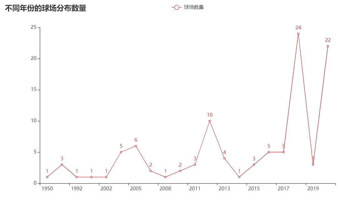
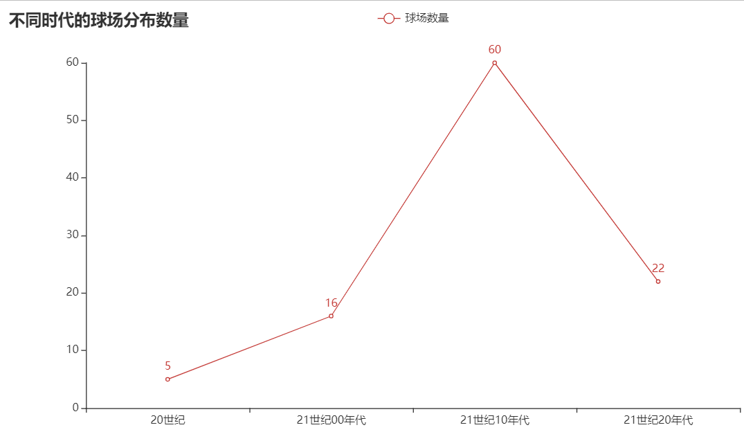
由图中可以看出厦门市中随时间的增加球场建造数量也在增加。
4.不同区球场建造数量(Count)与建造时间(BuildTime)的关系
from pyecharts.charts import Line
import pandas as pd
from pyecharts import options as opts

file = pd.read_csv('./csv/CountTime_SortTime.csv')
columns = file['Build_Time']
columns = columns.tolist()
file1 = pd.read_csv('./csv/Siming_count_time.csv')
file2 = pd.read_csv('./csv/Huli_count_time.csv')
file3 = pd.read_csv('./csv/Haicang_count_time.csv')
file4 = pd.read_csv('./csv/Jimei_count_time.csv')
file5 = pd.read_csv('./csv/Tongan_count_time.csv')
file6 = pd.read_csv('./csv/Xiangan_count_time.csv')
data1, data2, data3, data4, data5, data6 = [], [], [], [], [], []

for j in range(1, 7):
    column = eval('file' + str(j))['Build_Time']
    column = column.tolist()
    data = eval('file' + str(j))['Count']
    data = data.tolist()
    k = len(column) - 1
    for i in range(len(columns) - 1, -1, -1):
        if columns[i] != column[k]:
            eval('data' + str(j)).append('0')
        else:
            # print(columns[i])
            eval('data' + str(j)).append(str(data[k]))
            k = k - 1
columns.sort(reverse=False)
columns = [str(x) for x in columns]
line = (
    Line()
        .add_xaxis(columns)
        .add_yaxis("思明", data1, is_smooth=True)
        .add_yaxis("湖里", data2, is_smooth=True)
        .add_yaxis("海沧", data3, is_smooth=True)
        .add_yaxis("集美", data4, is_smooth=True)
        .add_yaxis("同安", data5, is_smooth=True)
        .add_yaxis("翔安", data6, is_smooth=True)
        .set_global_opts(title_opts=opts.TitleOpts(title="不同地区球场分布"), )
        .render("./html/Address_Count_Time_line.html"))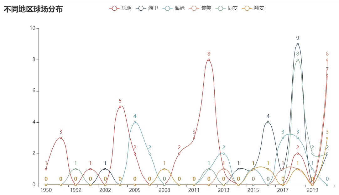
由图中可以看出厦门市中随时间的增加球场建造数量也在增加,尤其是在偶数年份。
5.厦门市球场建造数量(Count)与建造类型(Type)的关系
from pyecharts.charts import Bar
import pandas as pd
from pyecharts import options as opts
file = pd.read_csv('./csv/Type_SortCount.csv')
df = pd.DataFrame(file)
columns = []
data = []
for i in range(len(df)):
    document = df[i:i + 1]
    Type = document['Type'][i]
    Count = document['Count'][i]
    columns.append(Type)
    data.append(str(Count))
bar = (
    Bar()
    .add_xaxis(columns)
    .add_yaxis("球场数量", data)
    .set_global_opts(title_opts=opts.TitleOpts(title="不同类型的球场分布数量"))
    .render("./html/Xiamen_type_bar.html"))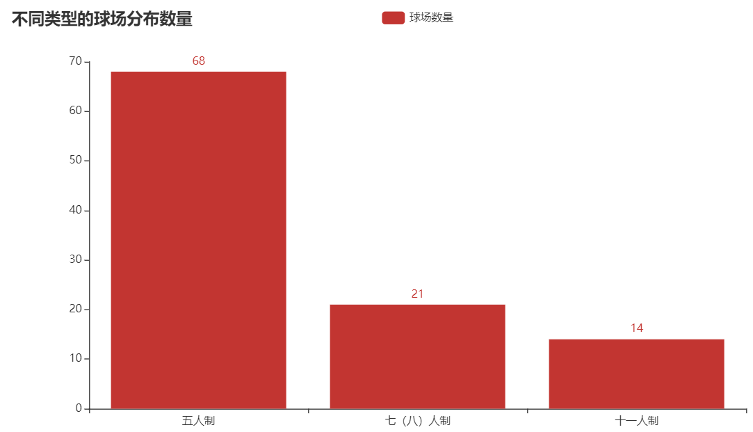
由图中可以看出厦门市中五人制球场类型最多,其次是七(八)人制,最少的是十一人制。
6.不同区球场建造数量(Count)与建造类型(Type)的关系
from pyecharts import options as opts
from pyecharts.charts import Pie
from pyecharts.commons.utils import JsCode
import pandas as pd
file1 = pd.read_csv('./csv/Count_Type_Siming.csv')
file2 = pd.read_csv('./csv/Count_Type_Huli.csv')
file3 = pd.read_csv('./csv/Count_Type_Jimei.csv')
file4 = pd.read_csv('./csv/Count_Type_Haicang.csv')
file5 = pd.read_csv('./csv/Count_Type_Tongan.csv')
file6 = pd.read_csv('./csv/Count_Type_Xiangan.csv')
column = file1['Type']
column = column.tolist()
data = []
for i in range(1, 7):
    d = eval('file' + str(i))['Count']
    d = d.tolist()
    data.append(d)
c = Pie(init_opts=opts.InitOpts(width="1700px",
                                height="750px"))
c.add("思明", [list(z) for z in zip(column, data[0])], radius=["30%", "40%"], center=[200, 220],
      rosetype='radius', label_opts=opts.LabelOpts(formatter=JsCode(fn), position="center"))  # 设置圆环的粗细和大小
c.add("湖里", [list(z) for z in zip(column, data[1])], radius=["30%", "40%"], center=[650, 220],
      rosetype='radius', label_opts=opts.LabelOpts(formatter=JsCode(fn), position="center"))  # 设置圆环的粗细和大小
c.add("集美", [list(z) for z in zip(column, data[2])], radius=["30%", "40%"], center=[1100, 220],
      rosetype='radius', label_opts=opts.LabelOpts(formatter=JsCode(fn), position="center"))  # 设置圆环的粗细和大小
c.add("海沧", [list(z) for z in zip(column, data[3])], radius=["30%", "40%"], center=[200, 600],
      rosetype='radius', label_opts=opts.LabelOpts(formatter=JsCode(fn), position="center"))  # 设置圆环的粗细和大小
c.add("同安", [list(z) for z in zip(column, data[4])], radius=["30%", "40%"], center=[650, 600],
      rosetype='radius', label_opts=opts.LabelOpts(formatter=JsCode(fn), position="center"))  # 设置圆环的粗细和大小
c.add("翔安", [list(z) for z in zip(column, data[5])], radius=["30%", "40%"], center=[1100, 600],
      rosetype='radius', label_opts=opts.LabelOpts(formatter=JsCode(fn), position="center"))  # 设置圆环的粗细和大小
c.set_global_opts(title_opts=opts.TitleOpts(title="不同区不同球场类型分布"))
c.set_series_opts(label_opts=opts.LabelOpts(formatter="{b}:{c}"))
c.render('./html/Address_count_type_Pine.html')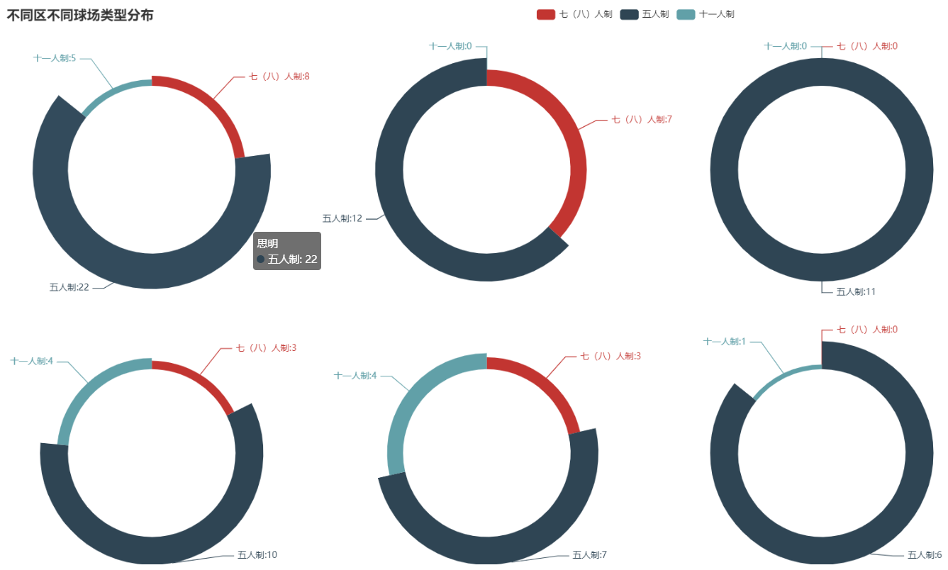
由图中可以看出厦门市中思明区,海沧区和同安区球场类型分布比较平均,湖里区无十一人制球场类型,集美区无十一人制和七八人制球场,翔安区无七八人制球场。
7.不同建造类型建造数量(Count)与建造时间(BuildTime)的关系
from pyecharts.charts import Line
import pandas as pd
from pyecharts import options as opts

file = pd.read_csv('./csv/CountTime_SortTime.csv')
columns = file['Build_Time']
columns = columns.tolist()
file1 = pd.read_csv('./csv/count_time_Five.csv')
file2 = pd.read_csv('./csv/count_time_Seven.csv')
file3 = pd.read_csv('./csv/count_time_Eleven.csv')
data1, data2, data3 = [], [], []
for j in range(1, 4):
    column = eval('file' + str(j))['Build_Time']
    column = column.tolist()
    data = eval('file' + str(j))['Count']
    data = data.tolist()
    k = len(column) - 1
    for i in range(len(columns) - 1, -1, -1):
        if columns[i] != column[k]:
            eval('data' + str(j)).append('0')
        else:
            # print(columns[i])
            eval('data' + str(j)).append(str(data[k]))
            k = k - 1
columns.sort(reverse=False)
columns = [str(x) for x in columns]
line = (
    Line()
        .add_xaxis(columns)
        .add_yaxis("五人制", data1, is_smooth=True)
        .add_yaxis("七(八)人制", data2, is_smooth=True)
        .add_yaxis("十一人制", data3, is_smooth=True)
        .set_global_opts(title_opts=opts.TitleOpts(title="不同类型球场分布"))
        .render("./html/Type_Count_Time_line.html"))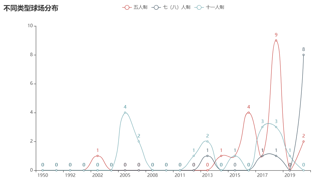
由图中可以看出不同球场类型大致都随时间的增加建造数量也在增加,而05年左右也增加了建造数量,推测是因为08年奥运会的原因。