
【版权声明】版权所有,严禁转载,严禁用于商业用途,侵权必究。
作者:厦门大学 2021级研究生 温宗恒
指导老师:厦门大学数据库实验室 林子雨 博士/副教授
相关教材:林子雨、郑海山、赖永炫编著《Spark编程基础(Scala版)》
【查看基于Scala语言的Spark数据分析案例集锦】
本案例针对Google Play应用商店数据进行分析,采用Scala为编程语言,采用Hadoop存储数据,采用Spark对数据进行处理分析,并对结果进行数据可视化。
一、实验环境
Ubuntu 20.04 LTS
Python 3.8
Hadoop 3.1.3
Scala 2.12.15
Spark 3.2.0
二、数据集
实验数据集采用kaggle的Google Play Store Apps数据集,该数据集包含googleplaystore.csv和googleplaystore_user_reviews.csv两个csv文件。可以从百度网盘下载数据集(提取码:ziyu)。本实验使用googleplaystore.csv文件,数据集包含字段如表1所示。
三、数据预处理
数据预处理主要是去除重复条目及处理异常值,并删除非必要的字段。
首先启动Hadoop的HDFS,将csv文件上传到HDFS文件系统中,然后启动spark-shell。
/usr/local/Hadoop/sbin/start-dfs.sh
hdfs dfs –put googleplaystore.csv
spark-shell
在spark-shell中读入csv文件
var raw = spark.read.option("header", true).csv("googleplaystore.csv")1)、删除重复数据
统计总行数,发现有重复的行,因此去掉重复行
输出:total rows: 10841, distinct rows: 10358
println("total rows: " +  raw.count() +", distinct rows: " +  raw.distinct().count())
raw = raw.distinct()
由于应用名称是唯一的,但是统计发现有大量的行里面的App字段重复,因此去掉App字段重复的行。
输出:Long = 523
raw.groupBy("App").count.filter("count > 1").count()
var distinct = raw.dropDuplicates("App")
2)、删除非必要字段
该数据集中,Size, Current Ver, Android Ver 字段中许多值为”Varies with device”,因此将这些字段舍弃,同时Genres与Category有重复,仅保留Category。最后将Last Updated字段也删除。
var df = distinct.drop("Size", "Last Updated", "Current Ver", "Genres", "Android Ver")3)、各字段异常值处理及数据格式转换
//Category
df.select("Category").distinct().collectAsList()
df = df.filter(not(col("Category").contains("1.9")))

//Rating
df.select("Rating").distinct().collectAsList()
df.groupBy("Rating").count().sort($"Rating".desc).show()
df = df.filter(col("Rating").contains(".") || col("Rating") === "NaN").withColumn("Rating", col("Rating").cast("float"))

//Reviews
df.filter(col("Reviews").isNull || col("Reviews") === "").count()
df.filter(col("Reviews").rlike("[^0-9]{1,}")).count()
df = df.withColumn("Reviews", col("Reviews").cast("int"))

//Installs
df = df.withColumn("Installs", regexp_replace(col("Installs"), "[^0-9]", "")).withColumn("Installs", col("Installs").cast("int"))

//Type
df = df.filter(not(col("Type") === "NaN"))

//Price
df = df.withColumn("Price", regexp_replace(col("Price"), "[$]", "").cast("float"))
Category字段中有异常值1.9,将其剔除。Rating字段也有异常值,同时有大量值为NaN的空缺值,将其全部删除或者用平均值代替均不合适,因此选择忽略,仅剔除异常值,然后转换为float类型。Reviews字段无空值或异常值,直接将其转换为int类型。同样的,Installs字段将特殊符号去除,仅保留数字,然后转换为int。Type字段存在一个异常值,将其去除。Price字段将$符号删除后转换为float。
四、数据分析
(一)、总体情况
1)、各个类别的App的数量
先对应用按类别进行分组操作,然后计算各分组的总数即得到各类别的App数量,为方便可视化,还进行了排序操作,最后将结果保存为csv文件。
df.groupBy("Category").count().sort(col("count").desc).toDF().write.option("header", true).csv("results/category_count.csv")2)、App评分分布
App的评分分布在0-5分之间,首先将评分划分为 [0, 3.0), [3.0, 3.5), [3,5, 4.0), [4.0, 4.5), [4.5, 5.0] 5个区间,然后统计落到各评分区间的应用个数即得到评分分布。
df.withColumn("Rating",
    when($"Rating" >= 4.5, lit("[4.5, 5.0]"))
    .when($"Rating">=4 && $"Rating"<4.5, lit("[4.0, 4.5)"))
    .when($"Rating">=3.5 && $"Rating"<4, lit("[3.5, 4.0)"))
    .when($"Rating">=3 && $"Rating"<3.5, lit("[3.0, 3.5)"))
    .otherwise(lit("[0,3)")))
    .groupBy("Rating").count().sort($"Rating".desc)
    .write.option("header", true)
    .csv("results/rating_distrib.csv")
3)、App评论数分布
评论数分布的计算与评分分布计算类似,首先将评论数划分为0, (0, 100), [100, 10000), [10000, 1000000), [1000000, ∞) 5种情况,然后统计各种情况的个数。
df.withColumn("Reviews", when($"Reviews" >= 1000000, lit("1M+"))
    .when($"Reviews">= 10000 && $"Reviews"<1000000, lit("10K+"))
    .when($"Reviews">=100 && $"Reviews"<10000, lit("100+"))
    .when($"Reviews">0 && $"Reviews"<100, lit("0+"))
    .otherwise(lit("0")))
    .groupBy("Reviews").count().sort($"Reviews".desc)
    .write.option("header", true)
    .csv("results/reviews_distrib.csv")
4)、App安装量分布
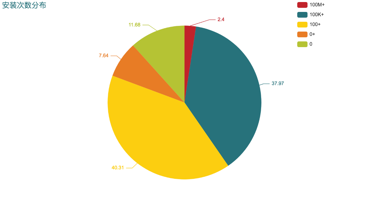
与上面一样,先将安装量划分为0, (0, 100), [100, 100000), [100000, 100000000), [100000000, ∞) 5档,然后统计各档的数量。
df.withColumn("Installs",
    when($"Installs" >= 100000000, lit("100M+"))
    .when($"Installs"> 100000 && $"Installs"<100000000, lit("100K+"))
    .when($"Installs">=100 && $"Installs"<100000, lit("100+"))
    .when($"Installs">0  && $"Installs"<100, lit("0+"))
    .otherwise(lit("0")))
    .groupBy("Installs").count()
    .sort($"Installs".desc)
    .write.option("header", true)
    .csv("results/installs_distrib.csv")
5)、安装量超过1亿的App
要获得安装量超过1亿的App,只需通过select操作即可实现
df.select($"App", $"Installs").where($"Installs" >= 100000000)
  .write.option("header", true).csv("results/top_installs.csv")
6)、各类别中安装量前5的App
要筛选出各类别安装量前5的App,首先需要创建一个临时视图。然后创建一张使用按类别分区并按安装量降序排序,并使用排序开窗函数添加了行号这一列的临时表,再从临时表中选出行号小于等于5的行。
df.createTempView("view")
spark.sql("select App, Installs from " + "(select *, row_number()" + " over (partition by Category order by Installs desc) " + "as rn from view) as tmp where tmp.rn <= 5").write.option("header",true).csv("results/top_5_install_each_category.csv")
7)、免费App与付费App评分、评论数、安装量对比
对比免费应用和付费App在各方面的情况通过分组再统计对应值即可实现,需要注意的是Reviews字段存在NaN,因此需要先丢弃这些数据再进行计算
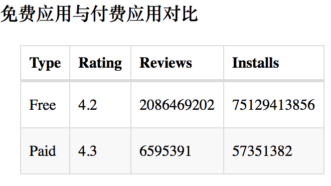
df.na.drop().groupBy("Type").agg(round(avg("Rating"), 1) as "Rating",sum("Reviews") as "Reviews", sum("Installs") as "Installs").write.option("header", true).csv("results/free_vs_paid.csv")(二)、关系分析
8)、付费App价格与评论数和安装量的关系
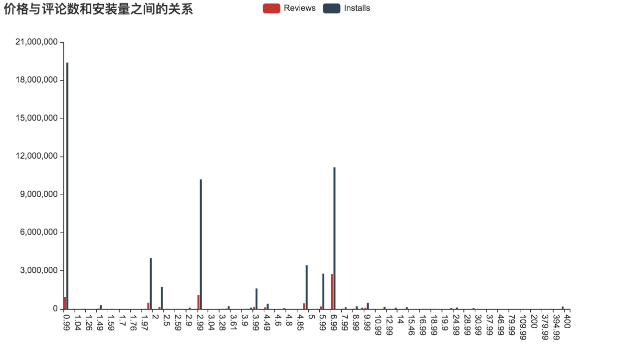
分析付费App的价格和评论数与安装量的关系通过筛选出付费App再计算相关的值即可
df.filter($"Type" === "Paid").groupBy("Price").agg(sum("Installs") as "Installs", sum("Reviews") as "Reviews").sort($"Price".asc).write.option("header", true).csv("results/price_reviews_installs.csv")9)、App的评论数与安装量之间的关系
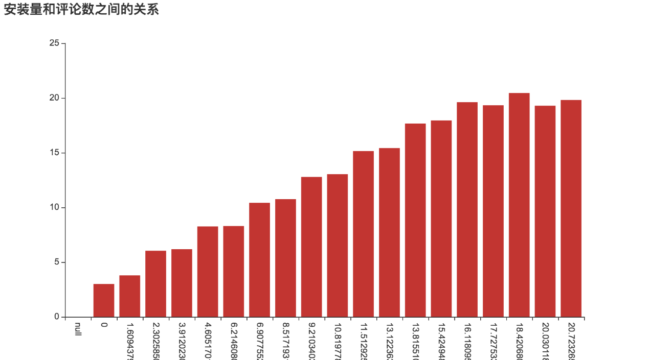
将数据按安装量进行分组,在计算各组的评论总数即可获得其关系
df.groupBy("Installs").agg(sum($"Reviews") as "Reviews").sort($"Installs".asc).write.option("header", true).csv("results/reviews_installs.csv")10)、用户评分与评论数和安装量之间的关系
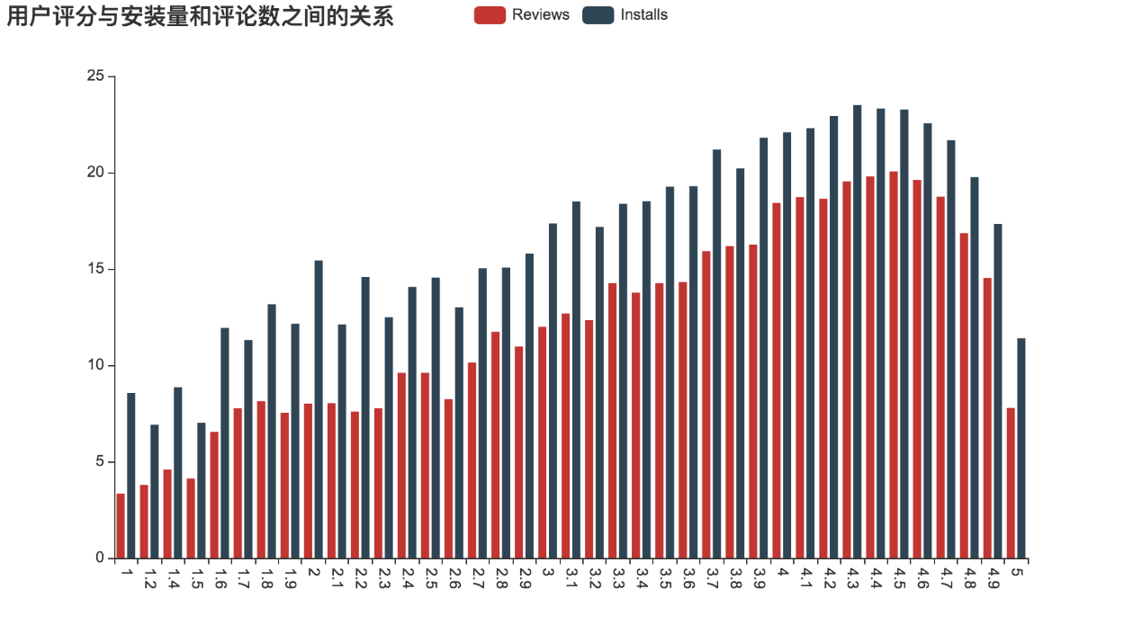
首先对数据按用户评分进行分组,然后分别统计各组的评论数和安装量的总数,就可以得到它们的关系。
df.groupBy("Rating").agg(sum($"Reviews") as "Reviews", sum($"Installs") as "Installs").sort($"Rating".asc).write.option("header", true).csv("results/rating_reviews_installs.csv")五、结果可视化
分析结果可视化采用pyecharts,ECharts的Python版本。同时使用Pandas进行数据的读取。为了导出图片,需要安装snapshot-selenium库,并下载ChromeDriver放在工程目录下。开发环境为JupyterLab。使用以下命令安装依赖库
pip3 install pyecharts, numpy, pandas, snapshot-selenium然后将数据取回本地
1.mkdir results
2.hdfs dfs -get results/*.csv
可视化代码如下
import glob
import numpy as np
import pandas as pd
from pyecharts.charts import Bar, Scatter, Pie, WordCloud
from pyecharts.components import Table
from pyecharts import options as opts
from pyecharts.globals import CurrentConfig, NotebookType, SymbolType, ThemeType
CurrentConfig.NOTEBOOK_TYPE = NotebookType.JUPYTER_LAB
# 导入输出图片工具
from pyecharts.render import make_snapshot
# 使用snapshot-selenium 渲染图片
from snapshot_selenium import snapshot
import os
if not os.path.exists("img"):
os.mkdir("img")
.# 各个类别的App的数量
category_count = pd.read_csv(glob.glob('results/category_count.csv/*.csv')[0])
bar_category_count = (
Bar(init_opts=opts.InitOpts(theme=ThemeType.LIGHT))
.add_xaxis(category_count['Category'].tolist()[:10])
.add_yaxis("", category_count['count'].tolist()[:10])
.set_global_opts(xaxis_opts=opts.AxisOpts(axislabel_opts=opts.LabelOpts(rotate=-15)),title_opts={'text':'App数量最多的10个类别'})
)
# bar_category_count.render_notebook()
make_snapshot(snapshot, bar_category_count.render(), "img/category_count.png")
# App评分分布
rating_dist = pd.read_csv(glob.glob('results/rating_distrib.csv/*.csv')[0])
pie_rating_dist = (
Pie(init_opts=opts.InitOpts(theme=ThemeType.INFOGRAPHIC))
.add("", [list(z) for z in zip(rating_dist['Rating'].tolist(), rating_dist['count'].tolist())])
.set_series_opts(label_opts=opts.LabelOpts(formatter="{d}%"))
.set_global_opts(
title_opts=opts.TitleOpts(title="用户评分分布"),
legend_opts=opts.LegendOpts(type_="scroll", pos_left="80%", orient="vertical")
)
)
#pie_rating_dist.render_notebook()
make_snapshot(snapshot, pie_rating_dist.render(), "img/rating_dist.png")
# App评论数分布
review_dist = pd.read_csv(glob.glob('results/reviews_distrib.csv/*.csv')[0])
pie_review_dist = (
Pie(init_opts=opts.InitOpts(theme=ThemeType.INFOGRAPHIC))
.add("", [list(z) for z in zip(review_dist['Reviews'].tolist(), review_dist['count'].tolist())])
.set_series_opts(label_opts=opts.LabelOpts(formatter="{d}"))
.set_global_opts(
title_opts=opts.TitleOpts(title="评论数量分布"),
legend_opts=opts.LegendOpts(type_="scroll", pos_left="80%", orient="vertical")
)
)
#pie_review_dist.render_notebook()
make_snapshot(snapshot, pie_review_dist.render(), "img/review_dist.png")
# App安装量分布
install_dist = pd.read_csv(glob.glob('results/installs_distrib.csv/*.csv')[0])
pie_install_dist = (
Pie(init_opts=opts.InitOpts(theme=ThemeType.INFOGRAPHIC))
.add("", [list(z) for z in zip(install_dist['Installs'].tolist(), install_dist['count'].tolist())])
.set_series_opts(label_opts=opts.LabelOpts(formatter="{d}"))
.set_global_opts(
title_opts=opts.TitleOpts(title="安装次数分布"),
legend_opts=opts.LegendOpts(type_="scroll", pos_left="80%", orient="vertical")
)
)
# pie_install_dist.render_notebook()
make_snapshot(snapshot, pie_install_dist.render(), "img/install_dist.png")
# 安装量超过1亿的App
top_install = pd.read_csv(glob.glob('results/top_installs.csv/*.csv')[0])
top_install_list = list(top_install.itertuples(index=False, name=None))
wc_top_install = WordCloud()
wc_top_install.add('',top_install_list,shape=SymbolType.DIAMOND, word_size_range=[10, 25])
# wc_top_install.render_notebook()
make_snapshot(snapshot, wc_top_install.render(), "img/top_install.png")
# 各类别中安装量前5的App
top_5_install_each_category = pd.read_csv(glob.glob('results/top_5_install_each_category.csv/*.csv')[0])
top_5_install_each_category_list = list(top_5_install_each_category.itertuples(index=False, name=None))
wc_top_5_install = WordCloud()
wc_top_5_install.add('',top_5_install_each_category_list, shape=SymbolType.DIAMOND, word_size_range=[10, 25])
wc_top_5_install.render_notebook()
make_snapshot(snapshot, wc_top_5_install.render(), 'img/top_5_each_category.png')
# 免费App与付费App评分、评论数、安装量对比
free_vs_paid = pd.read_csv(glob.glob('results/free_vs_paid.csv/*.csv')[0])
table_free_vs_paid = Table()
headers=list(free_vs_paid.columns)
rows=[list(free_vs_paid.loc[index]) for index in free_vs_paid.index]
table_free_vs_paid.add(headers,rows)
#table_free_vs_paid.add(free_vs_paid.columns.tolist(), free_vs_paid.values)
table_free_vs_paid.set_global_opts(
title_opts=opts.ComponentTitleOpts(title="免费应用与付费应用对比")
)
table_free_vs_paid.render_notebook()
# 付费App价格与评论数和安装量的关系
price_reviews_installs = pd.read_csv(glob.glob('results/price_reviews_installs.csv/*.csv')[0])
bar_price_reviews_installs = (
Bar(init_opts=opts.InitOpts(theme=ThemeType.MACARONS))
.add_xaxis(price_reviews_installs['Price'].tolist())
.add_yaxis("Reviews", np.sqrt(price_reviews_installs['Reviews']).tolist())
.add_yaxis("Installs", np.sqrt(price_reviews_installs['Installs']).tolist())
.set_global_opts(xaxis_opts=opts.AxisOpts(axislabel_opts=opts.LabelOpts(rotate=-90)),title_opts={'text':'价格与评论数和安装量之间的关系'})
.set_series_opts(label_opts=opts.LabelOpts(is_show=False))
)
# bar_price_reviews_installs.render_notebook()
make_snapshot(snapshot, bar_price_reviews_installs.render(), 'img/price_reviews_installs.png')
# App的评论数与安装量之间的关系
reviews_installs = pd.read_csv(glob.glob('results/reviews_installs.csv/*.csv')[0])
bar_reviews_installs = (
Bar(init_opts=opts.InitOpts(theme=ThemeType.MACARONS))
.add_xaxis(np.log(reviews_installs['Installs']).tolist())
.add_yaxis("", np.log(reviews_installs['Reviews']).tolist())
.set_global_opts(xaxis_opts=opts.AxisOpts(axislabel_opts=opts.LabelOpts(rotate=-90)),title_opts={'text':'安装量和评论数之间的关系'})
.set_series_opts(label_opts=opts.LabelOpts(is_show=False))
)
# bar_reviews_installs.render_notebook()
make_snapshot(snapshot, bar_reviews_installs.render(), 'img/reviews_installs.png')
# 用户评分与评论数和安装量之间的关系
rating_reviews_installs = pd.read_csv(glob.glob('results/rating_reviews_installs.csv/*.csv')[0])
bar_rating_reviews_installs = (
Bar(init_opts=opts.InitOpts(theme=ThemeType.MACARONS))
.add_xaxis(rating_reviews_installs['Rating'].tolist())
.add_yaxis("Reviews", np.log(rating_reviews_installs['Reviews']).tolist())
.add_yaxis("Installs", np.log(rating_reviews_installs['Installs']).tolist())
.set_global_opts(xaxis_opts=opts.AxisOpts(axislabel_opts=opts.LabelOpts(rotate=-90)),title_opts={'text':'用户评分与安装量和评论数之间的关系'})
.set_series_opts(label_opts=opts.LabelOpts(is_show=False))
)
# bar_rating_reviews_installs.render_notebook()
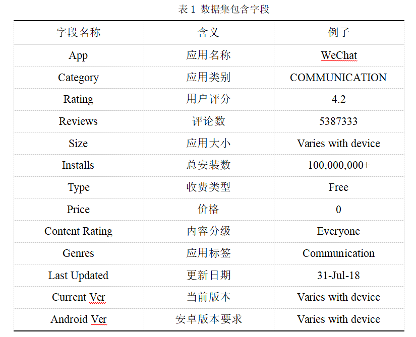
make_snapshot(snapshot, bar_rating_reviews_installs.render(), 'img/rating_reviews_installs.png')1)、App的数量最多的前10各类别
由于类别个数较多,仅显示前10个类别。从结果可以看出,数量最多的前三个类别分别是家庭、游戏和工具。
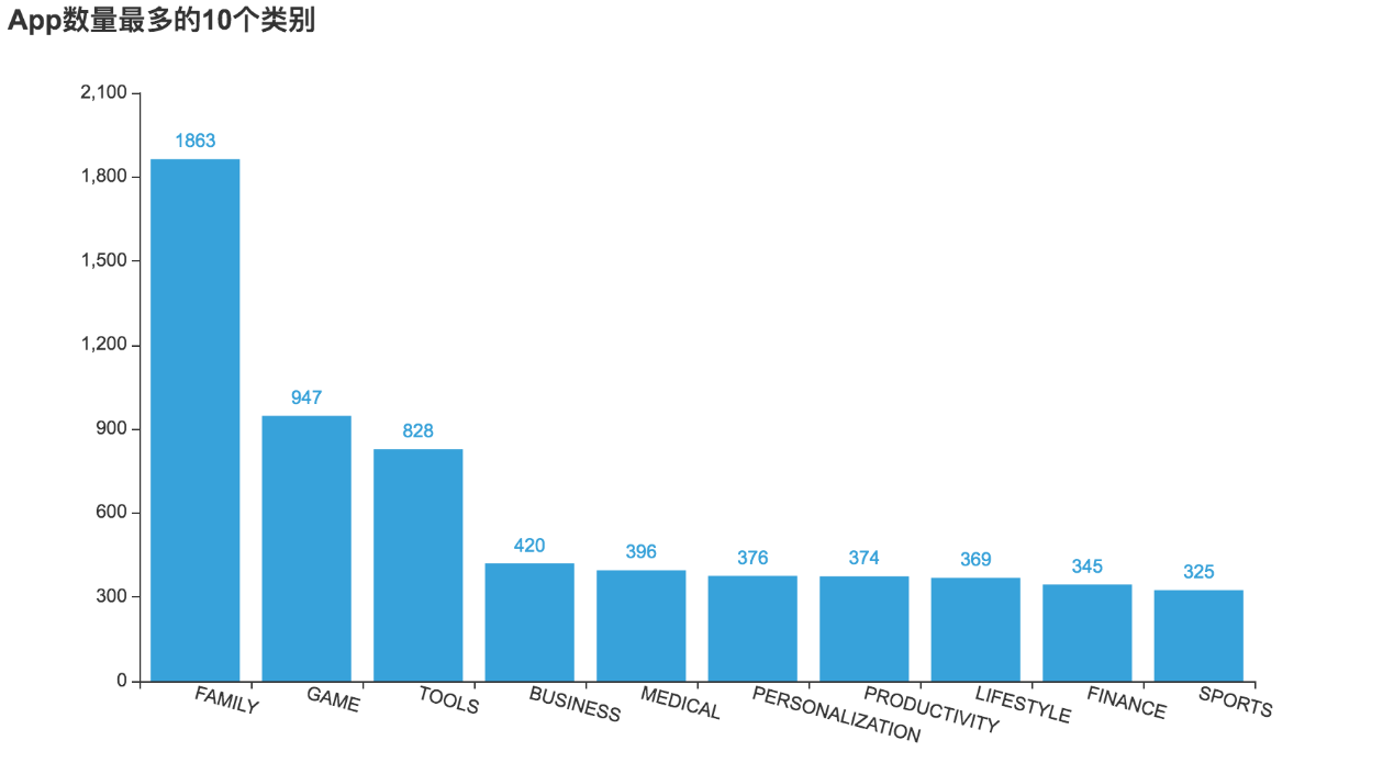
2)、App评分分布
从用户评分分布图可以看出,超过80%的App评分超过4.0,说明App的质量较高,用户整体较为满意
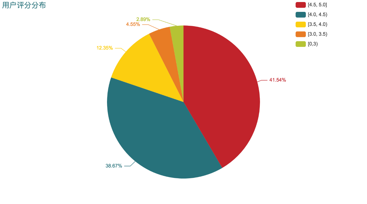
3)、App评论数分布
从评论数来看,大部分App的评论数为1百万以下,绝大部分App评论数介于100-1百万之间。
4)、App安装量分布
从App安装量分布图可以看出,安装量超过10亿的很少,安装量在100至10万之间的占比最多,其次为10万至10亿之间。
5)、安装量超过1亿的App
从词云图可以看出,安装量超过1亿的有很多是Google公司的产品,可能是由于系统预装的原因导致安装量高。同时,安装量超1亿的App都是常用的应用,如社交媒体应用和游戏。

6)、各类别中安装量前5的App
个类别安装量

7)、免费App与付费App评分、评论数、安装量对比
从表格中可以看出,虽然免费App安装量和评论数都比付费类App高,免费App数量更多是主要原因,但是付费App总体得分稍高于免费App,侧面可以反映出用户对付费类App也是较为满意。
8)、付费App价格与评论数和安装量的关系
从图中可以看出,0.99$的App安装量最大,其次是6.99$,10$以下的App占据了收费App绝大部分的安装量和评论数
9)、App的评论数与安装量之间的关系
由于评论数和安装量跨度很大,因此对两个坐标轴均取了对数,以更好地呈现结果。从图中可以看出,安装量和评论数呈现正相关的关系,安装量高的App评论数也高,符合现实情况。
10)、用户评分与评论数和安装量之间的关系
此处y轴也同样取对数。从关系图中可以看出,随着用户评分的升高,评论数和安装量也随之增加。
六、总结
该案例使用了Hadoop和Spark进行了数据分析,使用了Hadoop 的HDFS对数据进行存储,使用Spark Shell 对数据进行处理和分析,并对结果进行了保存,最后使用ECharts对分析结果进行可视化展示。
从分析结果可以发现家庭类App、游戏和工具类App是Google Play应用市场上数量最多的类别。过半App的评分大于4.0,说明质量能令用户满意。但大部分App的评论数都比较少,说明用户的评论意愿普遍较低,可以采取适当策略激励用户评论以更好地提高App质量。虽然数据来自Google Play应用商店,但是也可以给国内应用开发者一定的启发和建议。